Creating a user-friendly Data Validation in Excel Displaying help out of the way
Content
- Introduction
- Download
- Cell styles
- Proper labelling
- Data Validation
- A better way, no popup but help when needed
Introduction
I regularly design worksheets into which a user has to enter information. Of course when I do so, I make extensive use of:
- Cell styles
- Proper labelling
- Data Validation
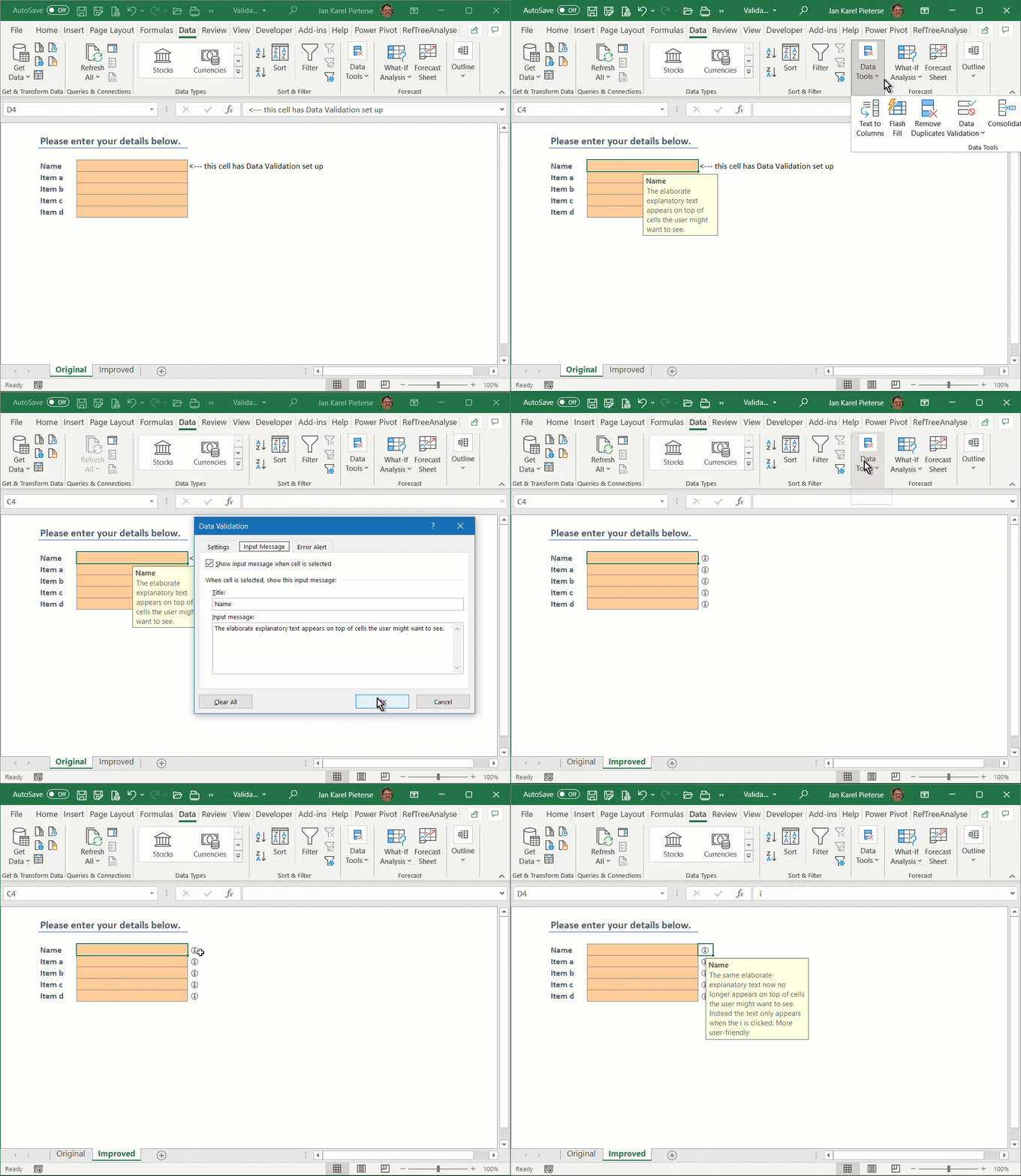
This post is mainly about leveraging the Data Validation Input Message. See the animated gif below:
Download
I prepared a sample workbook for you to download.
Cell styles
When you design a data entry form in Excel it is a good idea to use cell styles to clarify the purpose of the cells on the entry form and to direct the user to where his attention is needed.
A simple data entry form might look like this:
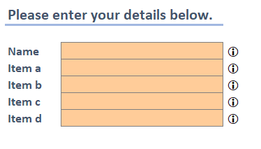
Looks nice doesn't it.
Note that I did not apply any manual formatting, I used the built-in cell styles:
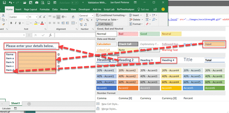
Now as happy I might be that Microsoft decided to provide some pre-defined styles, they didn't quite finish the job properly. Look at the formatting options of this "Input style":
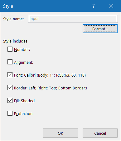
See what's wrong? No? They didn't set protection! So if I decide to password-protect my worksheet, all my input cells are locked. This is why I always add a user-defined style called "InputUnprotected". And perhaps a couple more if I need various different number formats to match what needs to be entered. One for each input type:
- InputUnprotectedNumber
- InputUnprotectedDate
- InputUnprotectedText
OK, enough about styles. Want to learn more? Read on about styles here.
Proper labelling
You might think this goes without saying, but I've seen plenty data entry sheets where it is left to the fantasy of the user what information is expected to go into which cells. My screenshot at the top lacks inspiration a bit, only the first cell is labelled more or less clear. Though you might argue that just asking for a name is ambiguous at best :-)
Data Validation
Now to the fun part of this article. Data Validation. Lets click the cell next to Name and open the DV dialog. Forget about its first tab for now, you already know what that one's for. In comes the "Input Message" tab!
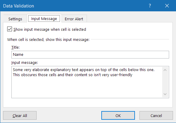
That looks pretty useful, does it not? You can set a Title and an Input message, with which you can show elaborate help! But there is a problem. It is elaborate and the message doesn't go out of the way:
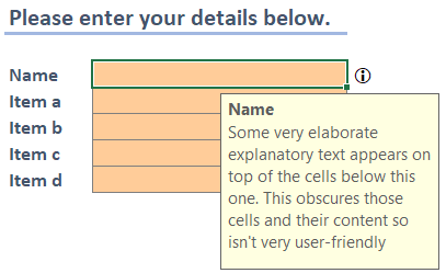
Also, the popup covers the remaining input cells and is very distracting, especially if the form contains many cells to fill. And it cannot be dismissed. You can drag it out of the way, but that causes all subsequent popup messages to appear in the same place. Luckily Excel does not save that position, so next time you open the file the popup appears in its nice in-your-face position again.
A better way, no popup but help when needed
I resolved that issue in my sample file in an interesting way, which I am sharing with you below. You did notice the tiny (i) "icons" next to the data entry cells, didn't you? Here is how I created them.
- Make sure there is an empty column next to your data entry cells
- Create a copy of the Heading 4 style (right-click, choose Duplicate)
- Name the new style i (yes just i, I'll explain below)
- change its properties so the Font tab looks like this:
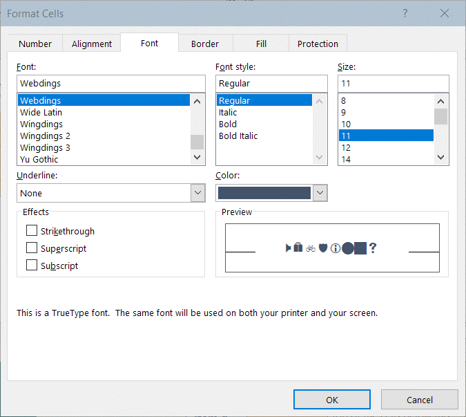
- Uncheck the Style's Locked box, we need to be able to click the cell.
- Now look at the Styles drop-down again:

Notice the nice i icon? The boxes in the Styles drop-down give an impression of what a cell looks like after applying the style. This includes the Font. If I would have used a regular name for this i style, the drop-down would have looked like this (I used 'SomeNameForTheStyle'):
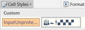
Given that the Webdings i character looks like the information icon I thought using i for its name might be good!
- So. Let's enter an i in the cells next to the entry cells. Then apply the new i style to them.
- Now select the first i-cell and open the Data Validation dialog and enter the pop-up information. Just like shown above.
- Also, to prevent people from changing the i to something else, setup
the first tab of the DV dialog to this:
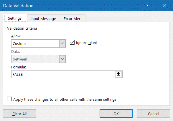
The FALSE formula prevents you from entering anything into the cell. That is how a custom formula in the Data Validation works: If the formula evaluates to TRUE (or 1), the entry is acceptable, otherwise it is not.
I know, I know, you can still hit the del key and the cell will be empty. Copying and pasting will also do its harm. But this is a good start.
Finally I want to add a nice touch to this new icon: I want to see this when my mouse passes over it:

This is done like so:
- Select the cell
- Click Insert, Link:
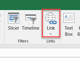
- Set it to these settings:
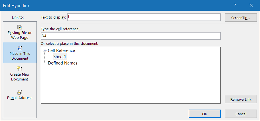
Note the Text to display and that the cell reference equals the cell I am adding the link to. We don't want Excel to jump to another cell, it should stay put. - Click the Screentip button and enter this:
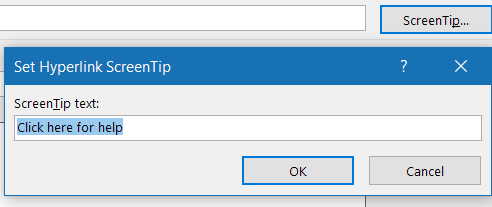
- Click OK twice.
- Curse because Excel changed the cell-style to Hyperlink so you have to re-apply the i-style again
You can avoid having to apply the cell style twice by reversing the order: first define the hyperlink, then set up the data validation and cell style.
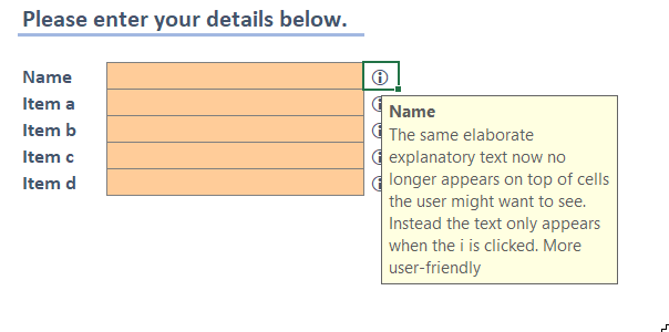
- Cheer, because now your data entry form looks like this if your
user clicks an i:

Comments
Showing last 8 comments of 14 in total (Show All Comments):Comment by: Karl Hoitsma (23-4-2018 20:43:01) deeplink to this comment
Nice work.
Thanks for presenting this; thanks for sharing.
Comment by: Jacques Raubenheimer (30-5-2018 03:46:51) deeplink to this comment
Great tip! Thanks.
The one limitation is the relatively sparse amount of text you can add in the data validation input message, but it does force one to think carefully about what to say.
You could improve the workflow by creating the hyperlink first, and then setting the style and the data validation, so that the style does not have to be re-set, although if you copy the cell to another point to save some time, then adjusting the hyperlink will require the style to be reset again.
Comment by: Jan Karel Pieterse (30-5-2018 10:32:25) deeplink to this comment
Hi Jacques,
Thanks for the tip!
Comment by: Andrew Engwirda (20-8-2021 03:40:00) deeplink to this comment
This is amazing Jan. It's great how you combine Data Validation, Hyperlinks and Webdings to set up a very professional "help" message. And I have to laugh at how the default Input style is set up with regards to protection. Oops!
Comment by: Jan Karel Pieterse (20-8-2021 16:05:00) deeplink to this comment
Hi Andrew,
Thanks!
Comment by: Helge Larsen (26-9-2022 21:43:00) deeplink to this comment
Really a good idea!
Since I expect to use it in the future, I have implemented it in VBA.
See the next two comments - because of the 2000 characters limit.
Comment by: Helge Larsen (26-9-2022 21:50:00) deeplink to this comment
Option Explicit
Sub HVL_Display_Cell_Info()
Const StName As String = "i"
Const aValue As String = "i"
Dim Answ As String
Dim Arr() As String
Dim aTitle As String
Dim N As Integer
Dim i As Integer
Dim aMess As String
Dim Addr As String
' Enter Help text
Answ = InputBox("Enter Title and Body Text!" & vbCr & vbCr & _
"Use backslash '\' to separate Title and Body Text" & vbCr & _
"and to separate individual lines in Body Text.", _
"Specify cell info")
If Answ = "" Then Exit Sub
Arr = Split(Answ, "\")
N = UBound(Arr)
aMess = ""
aTitle = Arr(0)
For i = 1 To N
If i > 1 Then aMess = aMess & vbLf
aMess = aMess & Arr(i)
Next i
If aMess = "" Then aMess = " "
' Make the special style
If Not HVL_Style_Exists(StName) Then HVL_Make_Special_Style (StName)
'Insert hyperlink
Addr = "'" & ActiveSheet.Name & "'!" & ActiveCell.Address(False, False)
ActiveSheet.Hyperlinks.Add Anchor:=ActiveCell, _
Address:="", _
SubAddress:=Addr, _
ScreenTip:="Click here for help", _
TextToDisplay:=aValue
' Cell value and style
ActiveCell.Value = aValue
ActiveCell.Style = StName
' Data validation used to display Help text
With ActiveCell.Validation
.Delete
.Add Type:=xlValidateCustom, _
AlertStyle:=xlValidAlertStop, _
Operator:=xlBetween, _
Formula1:="FALSE"
.IgnoreBlank = True
.InCellDropdown = True
.InputTitle = aTitle
.InputMessage = aMess
.ErrorTitle = ""
.ErrorMessage = ""
.ShowInput = True
.ShowError = True
End With
End Sub
Comment by: Helge Larsen (26-9-2022 21:51:00) deeplink to this comment
Function HVL_Style_Exists(ByVal aStyleName As String) As Boolean
Dim aStyle As Style
On Error GoTo ErrLab
Set aStyle = ActiveWorkbook.Styles(aStyleName)
On Error GoTo 0
HVL_Style_Exists = True
Exit Function
ErrLab:
On Error GoTo 0
HVL_Style_Exists = False
End Function
Sub HVL_Make_Special_Style(ByVal aStyleName As String)
Dim aStyle As Style
Set aStyle = ActiveWorkbook.Styles.Add(Name:=aStyleName)
With aStyle
.IncludeNumber = True
.IncludeFont = True
.IncludeAlignment = False
.IncludeBorder = False
.IncludePatterns = False
.IncludeProtection = True
.NumberFormat = "General"
With .Font
.Name = "Webdings"
.Size = 11
.Bold = False
.Italic = False
.Underline = xlUnderlineStyleNone
.Strikethrough = False
.ThemeColor = 4
.TintAndShade = 0
.ThemeFont = xlThemeFontNone
End With
.HorizontalAlignment = xlGeneral
.VerticalAlignment = xlBottom
.ReadingOrder = xlContext
.WrapText = False
.Orientation = 0
.AddIndent = False
.ShrinkToFit = False
.Borders(xlLeft).LineStyle = xlNone
.Borders(xlRight).LineStyle = xlNone
.Borders(xlTop).LineStyle = xlNone
.Borders(xlBottom).LineStyle = xlNone
.Borders(xlDiagonalDown).LineStyle = xlNone
.Borders(xlDiagonalUp).LineStyle = xlNone
With .Interior
.Pattern = xlNone
.TintAndShade = 0
.PatternTintAndShade = 0
End With
.Locked = False
.FormulaHidden = False
End With
End Sub
Have a question, comment or suggestion? Then please use this form.
If your question is not directly related to this web page, but rather a more general "How do I do this" Excel question, then I advise you to ask your question here: www.eileenslounge.com.