Styles in Excel
Content
- Introduction
- How styles work
- Creating styles
- Applying styles
- Deviate from a style
- Tips for using styles
- VBA examples and tools
- International issues
- Conclusion
Introduction
This article has also been published on Microsoft's MSDN site:
Using Styles to Dress Up Your Worksheets in Excel 2007
This article explains how you can use styles to ease maintenance of your spreadsheet models.
Microsoft has made it very easy to dress up your worksheets with all sorts of fill patterns, borders and other frills. Because formatting of cells is often done in an ad-hoc manner, many spreadsheet pages look messy.
By consistently using cell styles (instead of changing parts of the cell's formatting) you will be forced to think about the structure of your work. Religiously using styles may even force you to reconsider the overall structure of the entire spreadsheet model: The quality of the computational model itself may be positively affected.
I therefore consider Styles as being underused, underestimated and under exposed.
How styles work
A style is just a set of cell formatting settings which has been given a name. All cells to which a style has been applied look the same formatting-wise. When you change a part of a style, all cells to which that style has been applied change their formatting accordingly.
Use of styles takes some getting accustomed to, but may bring you great advantage. Imagine showing your nicely formatted sheet to your boss. Then your boss asks you if you could please change all input cells to having a light-yellow background fill, instead of a dark yellow one. For a large model, this may imply a huge amount of work. Would you have used styles, then it would have been a matter of seconds.
Styles are in fact an addition. Cell formatting is the sum of the applied style and all modifications to individual formatting elements on top of that style. What parts of the formatting options are included in a style is determined during the definition of the style (See screenshot below).
You access the style dialog from the Home Tab, Styles group, Cell Styles button:

Excel enables you to access the styles by clicking the dropdown next to
the styles gallery. The screen to create a new style looks like this (if
you click the New Cell Style option in the style gallery):
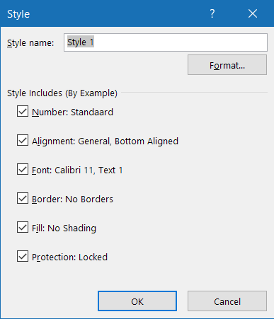
When you apply a style to a cell followed by another style, the end result will be an addition of the selected parts of both styles. What the end result of such an addition of styles will be, depends on which elements of both styles have been selected as being part of the style (this will be discussed later). Theoretically, this would have enabled us to use cascading styles, but unfortunately Excel does not keep a record of the order of applied styles. Only the last style is remembered. Also, styles can not be derived from other styles whilst maintaining a link to the parent style. Changes to the "original" style are not reflected in the "child" styles.
Creating styles
A convenient method to create a new style is by selecting a cell which has all formatting options in place which you want to incorporate in the new style. Select the cell and click the Home tab, click the New Cell Style button at the bottom of the Styles gallery.
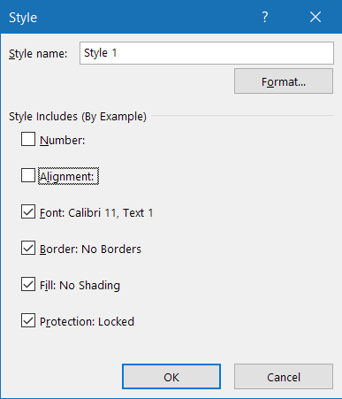
The Styles dialog screen.
To create a new style, simply type its name in the box "Style name". By default, all formatting elements are checked. Remove the checkmarks for the formatting elements you want to omit from the style you are creating (The dialog shown above has the Number and Alignment elements turned off).
Use the "Modify..." button to adjust the elements to your needs. Excel will show the standard "Format cells " dialog screen:
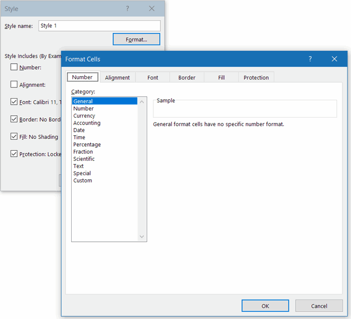
The format cells dialog screen, as shown after clicking Modify... on the Style dialog.
Note, that the elements in the Style dialog are identical to the tabs on the Format Cells dialog.
Note: As soon as you change a formatting element on a tab that was not selected on the Style dialog, Excel will automatically check that element for you; it will become part of that style.
Note that the style dialog will update/add the style, but the style will not be applied to the selected cells.
Applying styles
To apply a style to a cell, you simply click the Home tab and in the Styles group you Expand the Cell Styles gallery and click a style.
Deviate from a style
If you have applied a style to a set of cells and you change a formatting element of one of those cells, then modifications to that particular element of the style will no longer be applied to the modified cell.
So after changing a font attribute (like Bold) of a cell, changing the font attributes of the style will update all cells, except the one you just modified:
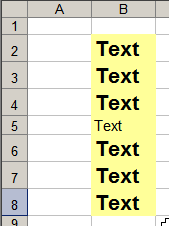
Series of cells with one style, 1 cell deviates from that style.
You can restore the style of a cell simply by selecting the cell and choosing the style from the style gallery.
Tips for using styles
Managing styles
If you like to keep an overview of what styles are available in your file I'd advise you to add a special worksheet to your workbook. Put the names of the styles in column A and an example output in column B:
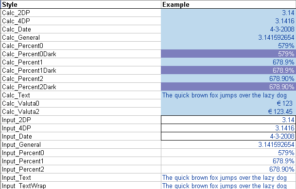
Table with styles in a worksheet
If you need to adjust a style, select the cell in column B and adjust the style settings from there.
Creating a new style based on an existing one is easy now: Just copy the applicable row and insert it anywhere in the table. Select the cell in column B of the newly inserted row and choose Home, Cell styles gallery, New Cell Style. Enter the name of the new style and click the Format button to change the style details. Don't forget to update the Style name in column A too.
Using styles
I advise you to use styles as strictly as you can. Avoid modifying one formatting element of a cell with a style. Instead, consider if it is worth the effort to add a new style. If for instance you have a style for percentage with 2 decimal places and you have a cell which requires three, then add a style for that purpose. You can thank me later.
Adapting this method will likely trigger you to think about what cell styles your document will need. By doing this your Excel models will gradually improve. You'll gain in consistency and loose the ad-hoc (often messy) formatting jungle.
Use functional sets of styles
By looking at your Excel model you will likely be able to categorise your workbook cells into various categories:
- Input cells
Cells that are the main input to your model - Parameter cells
Cells that contain constants for your model, such as boundaries. - Output cells
Cells in an area that is meant for output, such as printing or presenting the results of a calculation on screen. - Calculation cells
The cells where the actual calculation work is performed - Boundary cells
By shading otherwise empty cells you can easily make areas with differing functions stand out from other areas.
Consider creating styles for each of these cell functions, each (e.g.) having its own fill color. Don't forget to make decisions on whether or not a style's locked property needs to be on or off. If you use a system like this, it becomes very easy for you to maintain your file. Imagine how easy it now becomes to change a cell from an input to an output cell: you change its style. Done.
VBA examples and tools
The little VBA routines shown below will greatly easy your work with styles. As an important side effect, these also show you how the style object works in VBA.
Find cells with a certain style
This routine find cells with a style containing "demo" in its name:
Dim oSh As Worksheet
Dim oCell As Range
For Each oSh In ThisWorkbook.Worksheets
For Each oCell In oSh.UsedRange.Cells
If oCell.Style Like "*demo*" Then
Application.GoTo oCell
Stop
End If
Next
Next
End Sub
As soon as a cell is encountered with a style that matches that name filter, the code stops (Stop) and you can check out the cell in detail.
Creating a list of styles
This sub adds a table of your styles on a worksheet named "Config - Styles":
Dim oSt As Style
Dim oCell As Range
Dim lCount As Long
Dim oStylesh As Worksheet
Set oStylesh = ThisWorkbook.Worksheets("Config - Styles")
With oStylesh
lCount = oStylesh.UsedRange.Rows.Count + 1
For Each oSt In ThisWorkbook.Styles
On Error Resume Next
Set oCell = Nothing
Set oCell = Intersect(oStylesh.UsedRange, oStylesh.Range("A:A")).Find(oSt.Name, _
oStylesh.Range("A1"), xlValues, xlWhole, , , False)
If oCell Is Nothing Then
lCount = lCount + 1
.Cells(lCount, 1).Style = oSt.Name
.Cells(lCount, 1).Value = oSt.NameLocal
.Cells(lCount, 2).Style = oSt.Name
End If
Next
End With
End Sub
Clear all formatting of cells and re-apply their styles
The code below removes all formatting of all cells and subsequently re-applies their style to them.
Watch out: if you have not adhered to using styles strictly, you may lose all formatting in your file!!!
'Resets styles of cells to their original style (resets all formatting done on top of ANY style)
Dim oCell As Range
Dim oSh As Worksheet
If MsgBox("Proceed with care:" & vbNewLine & vbNewLine & _
"This routine will erase all formatting done on top of the existing cell styles." & vbNewLine & _
"Continue?", vbCritical + vbOKCancel + vbDefaultButton2, GSAPPNAME) = vbOK Then
For Each oSh In ActiveWindow.SelectedSheets
For Each oCell In oSh.UsedRange.Cells
If oCell.MergeArea.Cells.Count = 1 Then
oCell.Style = CStr(oCell.Style)
End If
Next
Next
End If
End Sub
Replace one style with another
The code below uses a list with two columns. The column on the left contains the names of existing styles. The column to its immediate right contains the names of the style you want to replace them with.
The code will run through the selected cells in the left column and check if the style name in the column to its right differs. If so, it will prompt you with the alternative name. Clicking OK will cause the code to update ALL cells to which the old style was applied to the new style. Before running this sub you need to select the cells in the left hand column.
'-------------------------------------------------------------------------
' Procedure : FixStyles
' Company : JKP Application Development Services (c)
' Author : Jan Karel Pieterse
' Created : 4-10-2007
' Purpose : Replaces styles with the replacement style as defined by a two column list.
' column 1 should contain the existing style, col 2 the replacing style
'-------------------------------------------------------------------------
Dim sOldSt As String
Dim sNewSt As String
Dim oSh As Worksheet
Dim oCell As Range
Dim oSourceCell As Range
Set oSourceCell = ActiveCell
While oSourceCell.Value <> ""
sOldSt = oSourceCell.Value
sNewSt = InputBox("Please enter replacement style for:" & sOldSt, "Style changer", oSourceCell.Offset(, 1).Value)
If sNewSt = "" Then Exit Sub
If sNewSt <> "" And sNewSt <> sOldSt Then
For Each oSh In ThisWorkbook.Worksheets
For Each oCell In oSh.UsedRange
If oCell.Style = sOldSt Then
Application.GoTo oCell
On Error Resume Next
oCell.Style = sNewSt
End If
Next
Next
End If
Set oSourceCell = oSourceCell.Offset(1)
Wend
End Sub
Removing formating from an Excel Table
Suppose you have just converted a range to a table (see this article), but the range had some formatting set up such as background fills and borders. Tables allow you to format things like that automatically, but now your preexisting formatting messes up the table formatting. One way to overcome this is by changing the style of the cells in the table back to the Normal style. This however removes your number formats too. The little macro below fixes that by first making a copy of the normal style, setting its Number checkbox to false and then applying the new style without number format to the table. Finally it applies the tablestyle and deletes the temporary style:
Dim oStNormalNoNum As Style
On Error Resume Next
Set oStNormalNoNum = ActiveWorkbook.Styles("NormalNoNum")
On Error GoTo 0
If oStNormalNoNum Is Nothing Then
ActiveWorkbook.Styles.Add "NormalNoNum"
Set oStNormalNoNum = ActiveWorkbook.Styles("NormalNoNum")
oStNormalNoNum.IncludeNumber = False
End If
With ActiveSheet.ListObjects(1)
.Range.Style = "NormalNoNum"
'Now apply tablestyle:
.TableStyle = "TableStyleLight1"
End With
ActiveWorkbook.Styles("NormalNoNum").Delete
End Sub
International issues
The VBA Style object offers both a Name and a NameLocal property. Which might give you the impression that if your Excel is set to Dutch, you can apply the Heading 1 style to a cell using this syntax:
Or perhaps like this:
But if my Excel is set to Dutch, trying to run that code yields this error:
Error 450; "Onjuist aantal argumenten of ongeldige eigenschappentoewijzing"
This is because the Heading 1 style's NameLocal property is the same as its Name property: Kop 1
Even worse, if you run through the Styles collection, the index of the Kop 1 style differs from the index of the Heading 1 style in an English Excel. They are sorted by their localized names, in alphabetical order. Moreover, if you haven't clicked any hyperlinks yet in your current Excel session, the Hyperlink and Followed Hyperlink styles are absent from the Styles collection altogether.
This is what the English and Dutch lists look like:
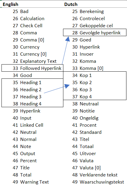
Notice how the Heading styles misalign with the Kop styles.
For workbooks (and add-ins) which need to work in several different language versions of Excel, my work-around for this issue is to have some cells in a (hidden) sheet somewhere (or inside the add-in), which have been formatted as Heading 1 to 4. The add-in then reads those cell styles to get the localized style name.
Conclusion
There is a lot to gain by using styles in your Excel work. To name but a few:
- Consistent formatting of your models
- Ease of maintenance
- A strict use of styles leads to a structured way of working
- Less problems with your file (There is a limit on how many different cell formats Excel can handle).
With this article I have tried to give insight in the use of styles in Excel. If you have comments, suggestions or questions, please don't hesitate to use the comment form below each page!
Download a pdf version of this article
Frequently asked Questions
What are the benefits of using styles in Excel worksheets?
What is the process to create a new style in Excel?
How can you apply a style to a cell in Excel?
What happens if you modify a formatting element of a cell that has a style applied?
What are some tips for managing and using styles effectively?
How can VBA be used to work with styles in Excel?
What international issues might arise when using styles in Excel VBA?
What are the key advantages of using styles in Excel models?

Comments