Charting a mathematical equation using Excel and defined names

Pages in this article

1. Introduction
2. Create the Chart
3. x-values
4. y-values
5. Sample Equations

Getting x values

The next task is to get a list if x values we can use for the x-axes of the chart. A little known fact, is that when a defined name is used to name a formula this formula will be an array formula by default. We're going to put that to use.

First we need a set of incrementing numbers. We'll use the ROW worksheet function for that.

When we define this name local to worksheet Sheet1:

Name: Sheet1!x

RefersTo: =ROW(1:20)

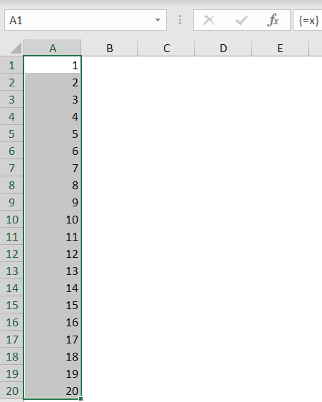
and we enter an array formula into cells A1:A20 (select A1:A20 in Sheet1 and type =x, then hit control-shift-enter) we get this result:

But we want the number of x-values to be dependent on a number entered into a cell. We'll use the OFFSET worksheet function for this purpose:

=ROW(OFFSET(Sheet1!$A$1,0,0,20,1))

If we replace the previous formula in "Sheet1!x" with the one above, the result will remain the same as shown above.
All it takes now is replace the fixed 20 with a cell reference:

=ROW(OFFSET(Sheet1!$A$1,0,0,Sheet1!$B$5,1))

Now we have the numbers 1 to 20 (or up to whatever number we enter into cell B5 on sheet1).

But we need more flexibility, we want to be able to set a minimum and a maximum value for x and use the 1-20 range to space out these limits.

Let's define these named ranges:

To get a series of "xNumberOfPoints" from xStart to xEnd, the following formula applies:

xPoint=xStart+xRange/(xNumberOfPoints-1)*Counter(1 to xNumberOfPoints-1)

So applying the approach depicted above:

=xStart+xRange/(xNumberOfPoints-1)*(ROW(OFFSET(Sheet1!$A$1,0,0,xNumberOfPoints,1))-1)

We'll name this new formula (surprisingly): Sheet1!x

Note:

Editing and creating names is much easier with the free Name Manager.