
Excel LAMBDA function, the basics
Content
- Introduction
- The LAMBDA function explained
- Example: the Quadratic formula
- Transforming into a true function
- Other examples
- Advanced formula environment
- Sharing lambdas
- Further reading
Introduction
In March 2021, Microsoft announced the new Excel LAMBDA worksheet function. This new function enables us to define custom functions which may replace UDFs currently written in VBA. These custom functions are powerful for two reasons:
- Any user capable of writing a cell formula can now define new functions
- Because it uses built-in functions and the built-in multi-threaded calculation engine, these new LAMBDA functions perform significantly better than VBA UDFs.
This page explains the basics of this new LAMBDA function and how you turn it into your very own custom named function.
Please note that for this function to work you need a Microsoft 365 license.
Download the accompanying file
The LAMBDA function explained
There are some good articles out there on the new LAMBDA function already:
From the Microsoft Research blog: LAMBDA: The ultimate Excel worksheet function
From Microsoft Excel Help: LAMBDA function
If you are familiar with the LET function, the structure of the new LAMBDA function will look familiar to you. In its simplest form it might look like this:
=LAMBDA(x,x^2)
All arguments but the last are inputs to the function, the last argument of LAMBDA is the calculation returning the final result. This means a LAMBDA formula always has one more argument than the number of input values it needs. In the example above, x is the input and x^2 is the returned result.
Example: the Quadratic formula
Anyone who has taken math at school has heard of the equation of a parabola
y=ax²+bx+c
and likely also of the Quadratic formula:
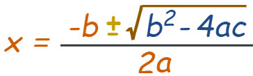
The Quadratic formula solves the problem of determining the intersections of a parabola with the x-axis (the roots of the equation).
In Math terms: it solves x in ax²+bx+c= 0 for given a, b and c.
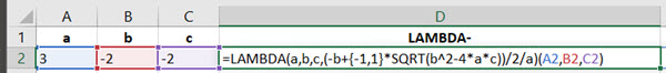
Translated to an Excel LAMBDA function, this looks like:
=LAMBDA(a,b,c,(-b+{-1,1}*SQRT(b^2-4*a*c))/2/a)
(the {-1,1} is Excel's way to get both results, it behaves as the +/- sign in the Quadratic Equation)
If you write this formula in a regular cell, Excel returns a rather unexpected result, a new Excel error code:
#CALC!
This is because we have not passed the required arguments to the formula. If placed in a cell like here, you must add the arguments -between brackets- behind the formula. Suppose our arguments are in cells A2, B2 and C2:
=LAMBDA(a,b,c,(-b+{-1,1}*SQRT(b^2-4*a*c))/2/a)(A2,B2,C2)
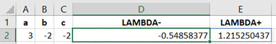
Which results in:
Transforming into a true function
By now you may be wondering what the fuss is about, this is still a (rather cumbersome looking) regular formula in a cell. Nothing fancy about it, now is it? But hold on, we'll get there. Open Excel's Name Manager (Formula tab, Name Manager button):
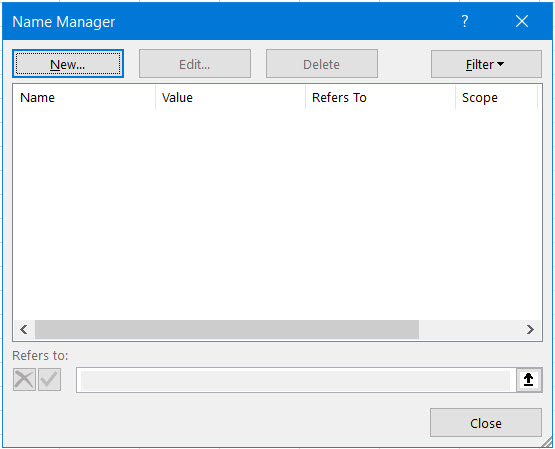
and click that "New..." button to add a new range name. Enter these details:
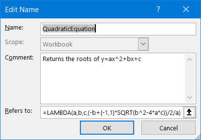
Notice how I also took the extra effort of entering a comment, I'll show you why later on. After OK-ing, you can now enter a formula like this into a cell:
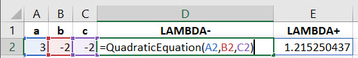
Presto! A new user-created function!
As promised, here's why entering a comment for the name is useful. Select any empty cell and start typing =Qua, Excel shows the autocomplete drop-down which includes that comment:
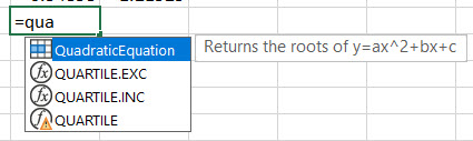
Now that is a great way to guide your users and tell them what the name is for!
Other examples
Other examples can be found here
Advanced formula environment
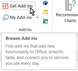
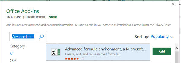
Microsoft has published a great tool to edit your Lambdas, called the Advanced Formula Environment. On your Insert tab, click "Get Add-ins":
Then search for "Advanced formula" and click 'Add' next to this entry:
Sharing lambdas
Download the accompanying file
So what is the story around sharing lambda functions with your co-workers? Copying Lambda formulas from one workbook to another is relatively easy. If you want to copy a lambda function from workbook A to B, make sure you add the lambda formula to any cell in the original file. Next, select both the cell with the lambda function and all of its precedent cells (the cells which are the lambda arguments, those the lambda uses for the calculation) and copy them. Now go to any empty area in your other workbook and paste-special, formulas. After the paste, you can clear the pasted cells. If a lambda function internally uses other lambda functions, those get copied into the other workbook too.
You can also share your lambdas by creating a public gist in github.
And you can use other people's gists by importing them using the Advanced Formula Environment add-in.
The QuadraticEquation lambda is available by importing this gist link into that add-in:
https://gist.github.com/jkpieterse/568a6e267fb54ff71adb66299b447e70
My water97 lambdas are available in this gist: https://gist.github.com/jkpieterse/9f2f1d30f188ca20e3311e83b5a2a8a5
And I have a useful SheetName Lambda too:
https://gist.github.com/jkpieterse/1541a4c51afa490958563fd7a9fdca0b
Further reading
I've also written an article on how to convert VBA UDF functions to a LAMBDA function.
Fellow MVP Mourad Louha wrote an excellent article about using lambdas for array manipulation.
Comments