Importing text files in an Excel sheet
Content
- Introduction
- Using Get & Transform Data (AKA Power Query)
- Automatically Opening CSV files as query
- Using the old text import wizard
- Refreshing your data
- Conclusion
Introduction
In this article I'll explain how to ease importing of .txt, .prn and/or .csv files into an existing sheet in Excel.
If you've ever tried to open a text file in Excel (File, Open, select "Text files" as the file type), you have probably used the old Text import wizard. If you have ever opened a CSV file by double-clicking the file in Windows, you have probably noted you can't set up how it gets imported. The text import wizard does not when these file are opened from a double-click. What if you have the situation where you get files with similar structure, which need the same text import settings over and over? How do you import the data from those files into the same worksheet each time, without having to re-define the import settings over and over again?
In this article I describe how to do this both using Get & Transform and the old-style text import wizard.
Using Get & Transform Data (AKA Power Query)
Before jumping into defining what the PowerQuery import steps are, you first need to ask yourself a couple of questions:
- Will the name of the file I am importing change?
- Will the location of the file change (regularly)
- Do I want to import one file, or perhaps more than one?
If the answer to 1 is yes, you may want to consider using different steps than described here. In such cases, consider using the From Folder option: Data tab, Get Data button, From File, From Folder. That route enables you to e.g. filter files by extension, maybe sort them so the most recent file is on top and then open only that file. Or you might want to open all .txt files in that folder which have a name starting with the word "balance". The possibilities are endless.
Anyway, let's import a single CSV.
Setting the locale
CSV files do not adhere to any international standards. The only thing that is certain is that in such a file columns are separated by a character. The same applies to other things in CSV files: There is no agreement on what exactly a date must look like, nor is there a standard for the decimal and thousands separators. All of this depends on the locale of the machine that generated the CSV. So you might have to deal with a CSV which is separated by semi-colons, has numbers using the comma as decimal separator and shows dates in the format dd-mm-yyyy. In the legacy text import wizard (shown below), you choose these settings after choosing the file. In PowerQuery it's easiest if you choose them up front.
It is a good idea to open your csv in Notepad so you can see what it contains. This allows you to find out things like
- Column separator
- Decimal separator
- Thousands separator
- Date format order

If you're lucky, the CSV you have has adhered to a system with settings taken from a known locale (unlike the example above). In that case you can first tell PowerQuery which locale to use when importing. Click the Data tab, select Get Data and click "Query Options". Then on the Regional Settings tab choose the correct "Locale":
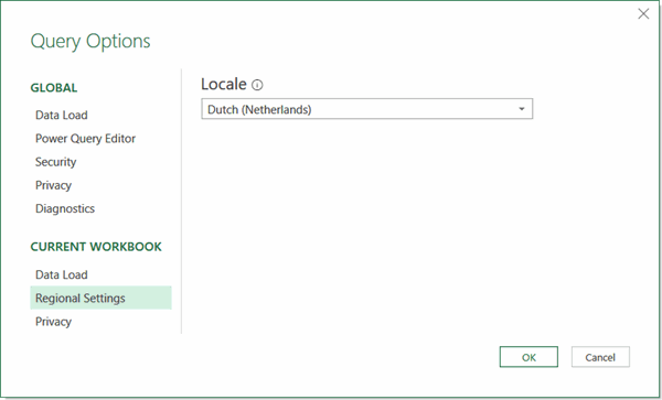
How do you decide which locale you need? The dialog does not tell you which separators and formats belong to each locale. Google to the rescue, Chris Webb has figured this out for us! Chris even made a workbook available which lists all of the formats.
Having set the locale we're now ready to start the actual import. Click Data, From Text/CSV. After choosing the file you want to import, this dialog opens.
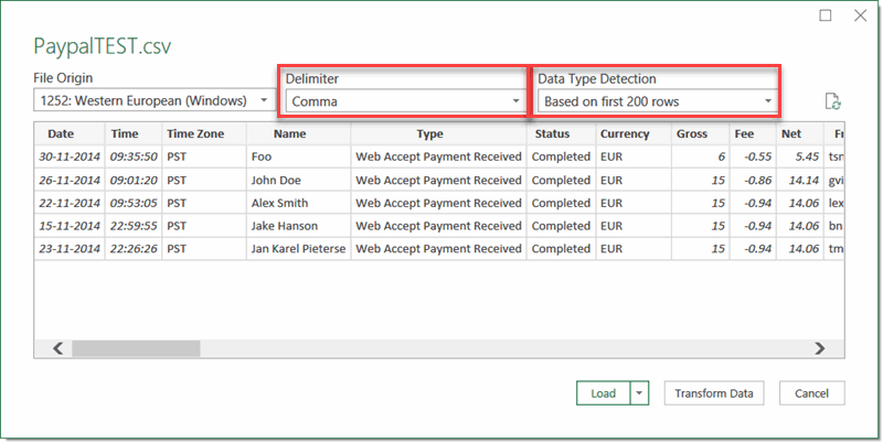
As you can see, Power Query has made a best guess on things like the delimiter of the file and has tried to defer the data types from the first 200 rows of data. Change those options if these are not to your liking.
The best step to take next is almost always to click "Transform Data". Simply clicking Load is hardly ever good enough as you'll have to retrace your steps if anything is amiss, like dates not being recognized as true dates. So always click Transform Data. You will thank me later.
After you've clicked Transform Data, the Power Query window opens. Check all your columns now. The icon next to their headers indicate the data type that was detected:

If any of the columns have the wrong datatype, click its icon to change it. You MUST choose the right data type, otherwise your data may be incorrect!
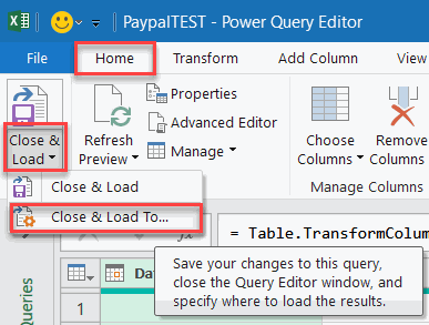
Now its the time to do things like deleting columns you don't need and sorting the data the way you want it sorted. Once you're happy with the data, click on the Home tab of the PQ ribbon and on the drop-down beneath "Close & Load", choose "Close & Load to..."
In the next dialog you get to decide where you want the resulting data from your query to go:
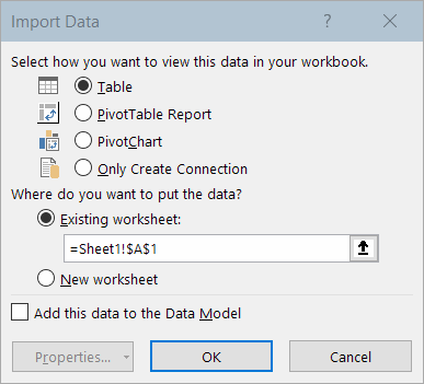
Unfortunately at this stage the Properties button is unavailable, click OK with these settings if you want the data to appear as a table in your worksheet.
To access those properties, click in the newly imported table, click the "Table Design" tab and find the Properties button:

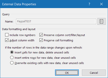
In the dialog that opens you can set things like what to do when less or more rows of data are imported and whether or not to adjust column widths automatically:
There are even more properties to modify, you find these additional properties by making sure the Queries & Connections pane is visible by clicking the appropriate button on the Data tab:
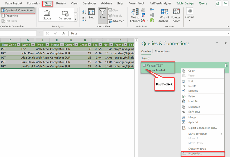
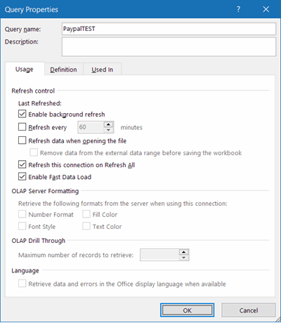
Then right-click on the highlighted query and select Properties to access properties like when the query must be refreshed:
Automatically Opening CSV files as query
If you double-click a CSV file in Windows, it is set to open in Excel automatically. However, oftentimes the CSV structure doesn't match your settings and the end result is a garbled unreadable mess. I've written a small add-in OpenCSVAsQuery which detects opening of CSV files and automatically transforms them into a new workbook with a table which imports the CSV using Power Query. You can set default import settings in the add-in using the button on the Data tab:

Using the old text import wizard
Getting back the old import wizards
As of Excel 2016, Power Query is built in to Excel. To promote usage of PowerQuery, the old-style text import wizard is hidden from the user interface. Here is how to get it back:
Click File, Options and click on the Data tab. Check the boxes you need as shown in the screen-shot:
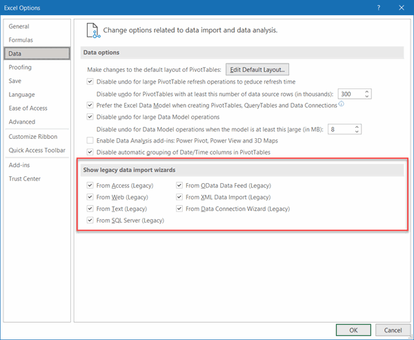
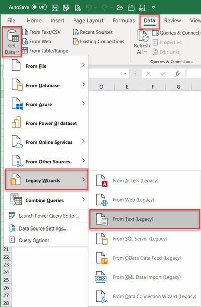
After that, you find the legacy Text import wizard here:
Selecting the file to import
First select the sheet where your data needs to appear. Note that the following steps differ for the various Excel versions.
On the ribbon, click the Data tab and then click Get Data, Legacy Wizards and finally "From Text (legacy)":

Select your file from the next dialog:
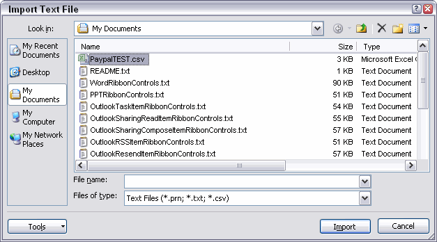
We've selected what to import. Now it is time to define what settings we need for the import.
Click the Import button. The text import wizard opens up:
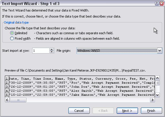
Step 1 of the Text Import Wizard, define file type.
In this example I have selected to import a delimited file and set the file origin to Windows (ANSI). Click Next when you're happy with the settings.
Step 2 of the wizard allows us to define the delimiters. I selected Comma:
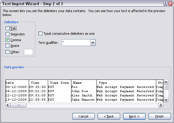
Step 2 of the Text Import Wizard: define delimiters
Click Next again to go into the third step, where you can select a format for each column of your file. I changed the date format of the first column to dmy order. Click a column to set up its formatting.
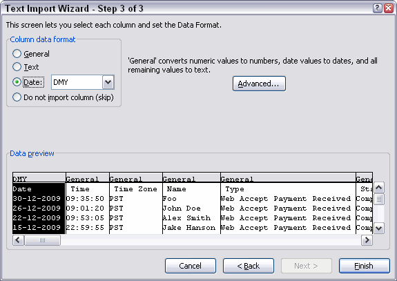
Step 3 of the wizard, Define column formats
You can click the advanced button to set up details like the decimal and thousands separators (note I switched them here):
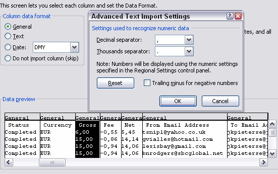
The Advanced text Import Settings dialog
Note that any changes made in this dialog apply to
all columns.
After you finished defining all columns, click the Finish button. Excel opens the Import Data dialog, asking where to put the results. Select the proper location.
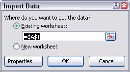
The Import Data dialog
Hold your horses, don't click OK yet! Click the properties button instead. The External Data Range Properties dialog opens up. There are some very important settings to be made here!
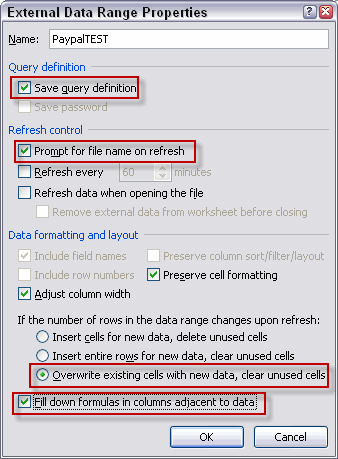
The External Data Range Properties dialog
Note that I have highlighted some important features in this dialog. I'll discuss them below.
Save Query Definition
We wouldn't want to redo the settings each time, so lets keep this one checked!
Prompt for the file name on refresh
Checking this box forces Excel to prompt you for a file name each time you hit the refresh button. Leave this box unchecked if you are importing the same file over and over.
Overwrite existing cells with new data, clear unused cells
What selection is best here depends on your needs entirely. The first two will force Excel to push existing data down and pull existing data up, depending on the size of your file.
I recommend NOT to put anything below an area where you are
importing data;
use a dedicated worksheet for this purpose.
Fill down formulas in columns adjacent to data
A very useful option. If you are planning to do calculations on each row, this option ensures each row of data will have your formulas.
Hit OK if you're happy with the settings.
Import your data
Finally, click OK to have your data imported. My sheet looks like this:

Results after importing the text file
Now that you have properly set up your import, save your file!
Refreshing your data
All of this was meant to predefine an import routine you have to do over and over again. So how do you import a new file? Easy. Click any cell within your sheet that holds data of a previous import.
On the Data tab, find the group called "Connections". Click the dropdown "Refresh All" and select "Refresh:
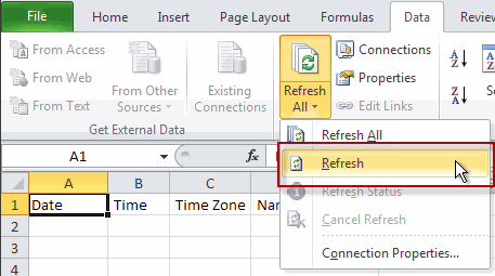
The Refresh All button on the ribbon
If you have set the option to prompt for a file, Excel will open the appropriate dialog. Select your file and click Import.
Conclusion
Importing text files into Excel can be a labor-intensive process if you're going through the same steps over and over again. With proper use of the data import options Excel offers, you can save yourself quite some work and at the same time improve consistency.
Whether you want to use the modern PowerQuery method or the old-school Text Import wizard is a matter of both personal preference and balancing the pros and cons of both methods. The legacy wizard makes it easy to select a different file on refresh. But the PowerQuery method offers way more flexibility in reshaping the data.
Feel free to add comments and/or questions below.
Frequently asked Questions
What types of text files can be imported into Excel using the methods described?
How can Power Query be used to import text files into Excel?
What should you consider about file names and locations when importing with Power Query?
How do you set the locale for importing CSV files in Power Query?
Why is it recommended to click "Transform Data" instead of just "Load" when importing?
How can you enable the old text import wizard in Excel 2016 and later?
What are the steps to import a text file using the old text import wizard?
What important settings can be configured in the External Data Range Properties dialog?
How do you refresh imported data when using the old text import wizard?
What are the advantages of using Power Query versus the old text import wizard?

Comments