Pivottable Slicers
Introduction
Pivottables are one of the most powerful data analysis features Excel has to offer. From version to version, Microsoft have added functionality to this feature. Pivottable Slicers were introduced with Excel 2010 and as of Excel 2013 you can also insert a slicer to filter a table. In this article I'll discuss how you can put slicers to work.
Content
- Why slicers
- Configuring Slicers
- Slicers and VBA
- Synchronising Slicers
- Show Selected Items
- Conclusion
- Sample files
- Other sources
Why Slicers
If you've ever done filtering on (Pivot) tables before you'll know why this can be a challenge. But I'll spell it out here in case you haven't.
With any version of Excel, you can filter the content of your table or Pivottable report (or pivot chart for that matter) by clicking the appropriate dropdown and checking/unchecking boxes:
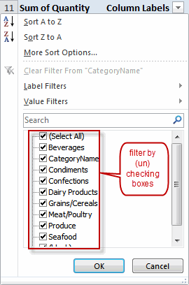
Old-style (Pivot) table filtering
This method has a number of drawbacks listed below, in no particular order:
- Users who are not familiar with (Pivot) tables are easily confused by the filter dropdowns.
- To check/uncheck an item you must click in the checkbox, clicking the item only selects the item, it does not change the check.
- You cannot drag across the items to select a number of them.
- You cannot modify the appearance of the filter, apart from changing the size of the entire box.
- There is no way of telling which filters are in effect, only that there is some filtering applied.
- If you have more than one Pivottable tied to the same data, then applying a filter to Pivottable 1 does not necessarily mean Pivottable 2 gets the same filter settings; it takes VBA to keep them in synch automatically.
- If your report has hierarchical data (countries and cities for example), then a filter on a higher level field in the hierarchy will not change the items visible in the lower fields. So Excel will happily show Toronto, even when you've unchecked Canada in the country filter. This makes filtering on large Pivottables very cumbersome.
Slicers put an end to a number of these problems:

Slicer filtering
- They are very intuitive to use.
- You can click an item, drag across a number of them, use control or shift click, in other words they are easier to use.
- The appearance of a slicer is very configurable.
- You can tie one slicer to as many Pivottables as you like, keeping them in sync (you cannot do this with table slicers).
- You can have multiple "copies" of a slicer operating together on different worksheets.
- Slicers reveal hierarchical data in a sensible manner: non-applicable values are shaded differently so you'll know they do not apply in the current filter mode.
Configuring Slicers
Slicer options on the ribbon
There is a host of settings you can apply to your slicers. The Ribbon shows most of them:
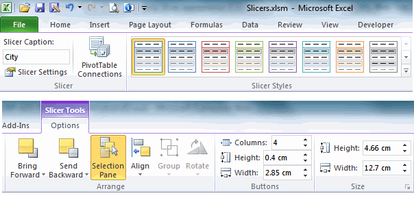
Ribbon (cut in two halves so it fits on this page) showing the slicer options
tab.
The Slicer Tools contextual ribbon tab houses a number of groups to change your slicer's appearance and behavior. Let me discuss them here.
Slicer group
This group houses three important controls. You can change the name of a slicer here (Slicer Caption), change some settings controlling which items are listed in a slicer and how they are sorted and filtered (Slicer Settings). Also, you can set up which Pivottables connect to your slicer (I explain that below).
Slicer Styles Group
A quick way to format your slicers is by applying one of the built-in slicer styles. Like any style in Excel 2010, these adhere to the theme you've selected. This makes it easy to keep your workbook design tidy and consistent.
Like cell styles you can create your own slicer styles too, by right-clicking one of them and choosing "Duplicate", followed by right-clicking the newly duplicated style and choosing "Modify".
Buttons group
Just like you can easily change the colors of your slicers by applying a different style to the slicer it is simple to modify the button layout and appearance, just adjust the numbers in that group of the ribbon.

These three controls enable you to change the button layout and size
Size group
And last but not least a small group which lets you edit the button sizes.
Commands not in ribbon
Unfortunately, not everything you need is on the ribbon. The missing options are quickly accessible through the slicer's right-click menu however. Select the "Size and Properties" option to get there. Here you can control whether or not the slicer must be printed and should move/size with cells just like any other shape on a sheet. And you can turn off resizing and moving to prevent your users from messing with your layout.
Changing a Slicer's font size
If you've scurried through all slicer dialogs like I have, you'll have noticed there is no way to change the font size of a slicer.
Or is there? Of course there is, but is has been cunningly hidden!
The basic idea is that you must edit the slicer's style. But since you can only edit custom styles, the first step is to add a custom style. Pick one you like best and right-click it, then select Duplicate...:
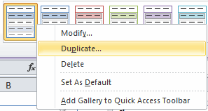
Right-click a slicer style and select "Duplicate"
The second step is editing the new custom style. Right-click that style and select "Modify...":
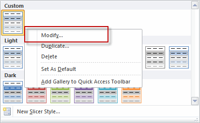
Right-click a slicer style and select "Modify".
In the dialog that pops up, select "Whole Slicer" end then click the Format button:
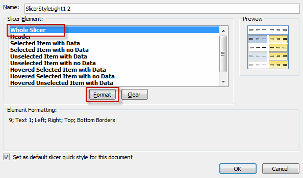
The Modify slicer Quick style dialog.
As you can see in the screenshot below, now you can edit the slicer's Font.
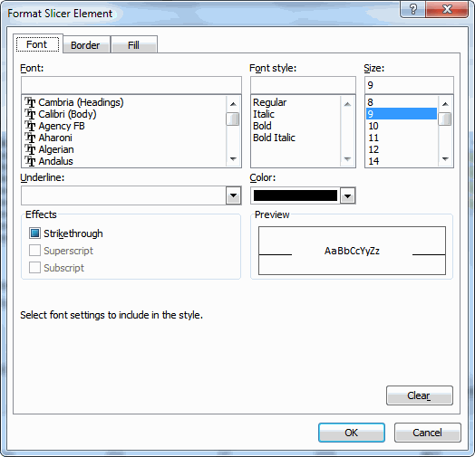
Time to select a nicer font for your slicer!.
After you OK this dialog, probably nothing appears to happen to your slicer. Don't worry, all that is needed now is applying your new custom style to the slicer and you're done!
Controlling which pivots are handled by your slicers.
A very useful option of slicers is that you can tie them to more than one Pivottable and/or -chart.
The way to handle this is by selecting the slicer in question and then clicking the Pivottable Connections button in the Slicer Settings group on the Slicer Tools contextual ribbon tab:
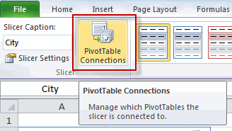
the Pivottable Connections button in the Slicer Settings group on the Slicer
Tools contextual ribbon tab.
This brings up the following tiny dialog:
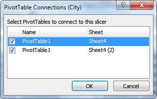
the Pivottable Connections dialog.
As you can see, Excel has listed a couple of Pivottables in your file to tie the slicer to.
Luckily, Excel is smart enough to ensure that only Pivottables using the same cache as the selected slicer is tied to are in the list.
If you have more than one slicer on a particular field (e.g. a slicer on "City" on each sheet with a Pivottable), then you must take care when selecting which tables the slicer relates to. As soon as you check more than one check box, the slicers working on the checked Pivottables will be permanently tied together. The only way to make the slicers work independently again is by using the Undo button.
Slicers and VBA
This chapter has also been published on The Microsoft Office Blog.
Juggling the SlicerCaches collection
For each slicer you add to your workbook, Excel adds a SlicerCache object too, which controls which Pivottable(s) your slicer controls.
So suppose we have a workbook with two Pivot caches. Pivotchache1 has two pivot tables: Pivottable1 and Pivottable2. As soon as you add a slicer to a Pivottable (even if the slicer ties to the same field of the Pivottable) you get a SlicerCache object tied to the pivotCache to which the pivot table belongs:
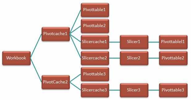
Hierarchy of the slicer and its family
Note that the above picture is not entirely correct. In the object model, PivotTables are in fact tied to a slicerCache, not to a slicer. But on the user interface side of things it is the slicer the user actually sees, which is why I put that in-between.
Also note that this is a diagram for pivot table slicers. A table slicer has a much simpler diagram where a table has one slicer cache with attached to that all slicers pertaining to that table. No other tables are involved.
The code below enumerates all slicer caches and their associated pivot tables in your workbook:
Dim oSlicer As Slicer
Dim oSlicercache As SlicerCache
Dim oPT As PivotTable
Dim oSh As Worksheet
For Each oSlicercache In ThisWorkbook.SlicerCaches
For Each oPT In oSlicercache.PivotTables
oPT.Parent.Activate
MsgBox oSlicercache.Name & "," & oPT.Parent.Name
Next
Next
End Sub
As soon as you check more than one Pivottable on the Pivottable Connections dialog of a Slicer, the slicers in question will share a single SlicerCache object. The other SlicerCache object will be removed from the collection. This explains why you cannot go back by unchecking all but one Pivottable in that dialog: all joined slicers will now be changed by changing the checked Pivottable(s) on any of them. In turn, each checked Pivottable becomes part of the Pivottables collection of the remaining SlicerCache object.
If you decide to select Slicer1 and change its pivot connections by checking both Pivottable1 and Pivottable2, one slicer cache is deleted (the one belonging to the Pivottable you checked to add to the current slicer). So the hierarchy changes to:
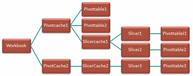
Changed hierarchy of slicers
So both Slicer1 and Slicer2 control Pivottables 1 and 2. The slicers 1 and 2 are in sync too because it is in fact the SlicerCache that is changed by the slicer. So the hierarchy in the picture above isn't entirely true.
Changing the buttons using VBA
It is easy enough to change the button appearance using a bit of VBA:
With ActiveWorkbook.SlicerCaches("Slicer_City2").Slicers("City 2")
.NumberOfColumns = 3
.RowHeight = 13
.ColumnWidth = 70
'Note that changing the ColumnWidth also affects the Width of the slicer itself
'So the next line will change the ColumnWidth!
.Width = 300
End With
End Sub
Note that the numbers do not coincide with what is shown on the ribbon. Apparently the unit of measure differs between VBA and the ribbon.
Changing the slicer itself and some SlicerCache properties
Changing some aspects of your slicer using VBA isn't hard to do. In fact, the macro recorder makes finding out how this works relatively simple. After changing some settings and doing a bit of tidying up I got:
With ActiveWorkbook.SlicerCaches("Slicer_City2").Slicers("City 2")
.Caption = "City"
.DisplayHeader = True
.Name = "City 2"
End With
With ActiveWorkbook.SlicerCaches("Slicer_City2")
.CrossFilterType = xlSlicerNoCrossFilter
'xlSlicerCrossFilterShowItemsWithDataAtTop:
' Visually indicate items with no data, items with data are pushed to the top
'xlSlicerCrossFilterShowItemsWithNoData:
' Visually indicate items with no data, items with no data stay put
'xlSlicerNoCrossFilter:
' No indication for items with no data.
.SortItems = xlSlicerSortAscending
.SortUsingCustomLists = False
.ShowAllItems = False
' This ensures that data no longer in the pivot cache is not shown on the slicer
End With
End Sub
Synchronising Slicers
Oftentimes a reporting workbook contains more than one pivot table. As I showed you already, synchronising pivot tables that use the same pivot cache is very easy if you tie them together with one or more slicers pointing to both pivot tables. You use the "Pivottable Connections" button on the ribbon for that.
However, it frequently happens that pivot tables do not share a pivot cache, but still need to be in sync, for instance if your slicer is filtering on a reporting period such as Year, Quarter or Month. In the code below I assume all pivot caches share the fieldnames to filter on. I also assume the tied-together slicer caches share the same values, in other words, all years appearing in Slicer_Year also appear in Slicer_Year1 and vice versa. If your situation differs (values in slicer cache 1 might be missing in slicer cache 2 or the other way around), you will need to take special precautions.
Setting things up
The first action needed is to make sure each slicer is connected to all relevant pivot tables belonging to its pivot cache. Take care NOT to add a pivot table to a slicer for which the field in question is not used in that pivot table, because a slicer can operate on a field that isn't included in the pivot table itself. It will filter your pivot table and the pivot itself gives no clue that it was filtered (other than the slicer).
Suppose you have three reports: Monthly, Quartely and Yearly. You might have three slicers for those pivot tables: Year, Month and Quarter. But for the quarterly and yearly pivot table, it makes no sense to tie them to the Month slicer. In fact, it would turn them all into a monthly report. In a situation like this, only the Year slicer is a sensible one to connect to all three pivot tables. If you would want to connect the Quarter slicer to the Month slicer, you would need some VBA which, after selecting a month, sets the associated Quarter in the Quarter slicer. The code below isn't that smart, it just syncs Year, Quarter and Month slicers, assuming you did all of the slicers pivot table connections correctly.
Triggering a change in a slicer filter
There is no event tied to slicer actions directly. However, clicking a slicer triggers the Workbook_SheetPivotTableUpdate event in the ThisWorkbook module (there is a similar event in the sheet modules, but I want one generic event which responds to any pivot table update). The empty event stub looks like this:
End Sub
Sh is an object variable pointing to the worksheet on which a pivot table just updated. Target is an object variable pointing to the pivot table that just updated.
The first thing the code needs to do is find out which slicers are connected to the pivot table that just changed and set a pointer to the ones we want to use to sync the other pivot tables to.
First, we declare some variables:
Dim oScKwrt As SlicerCache
Dim oScYear As SlicerCache
Dim oSc As SlicerCache
Dim oPT As PivotTable
Dim oSi As SlicerItem
The first three are going to hold the Year, Quarter and Month slicers tied to the changed pivot table. Note that no more than two of these three are in fact tied to the pivot table: either Year and Month, Year and Quarter or just Year.
Finding the slicer that was clicked
So now step through all SlicerCaches and then through all their associated pivot tables to find out which slicers are tied to the changed pivot table:
For Each oPT In oSc.PivotTables
If oPT.Name = Target.Name And oPT.Parent.Name = Target.Parent.Name Then
If oSc.Name Like "*Year*" Then
Set oScYear = oSc
ElseIf oSc.Name Like "*Month*" Then
Set oScMonth = oSc
ElseIf oSc.Name Like "*Quarter*" Then
Set oScKwrt = oSc
End If
Exit For
End If
Next
If Not oScYear Is Nothing And Not oScMonth Is Nothing And Not oScKwrt Is Nothing Then Exit For
Next
As you can see, we only pick up the slicers Month, Quarter and Year because those are the ones we want to sync.
Synchronising the slicers
Now that we have the slicer(s) that have been clicked, we want to sync them with slicers with similar names. By Default, Excel names SlicerCaches like this: Slicer_FieldName. If another slicer with the same fieldname is added (which adds a SlicerCache too), it is called Slicer_FieldName1, the next one is called Slicer_FieldName2 and etcetera. So what the code below does is loop through all slicer caches again, looking at their names to figure out which ones belong together.
The code has a special trick to avoid problems. Suppose you have a slicer which has its first item selected and the remaining items de-selected. Suppose that the sister slicer is clicked and we click the second item. When the code runs through all slicer items, it will start with the first one, which will be de-selected. This causes the slicer to select all items, because it is not allowed to de-select all items of a slicer. Subsequently the code runs through the remaining items and sets them as needed. The end result is that both item 1 and item 2 are selected, rather than just item 2. The trick around this is setting the last slicer item to "Selected" before running through the loop:
For Each oSc In ThisWorkbook.SlicerCaches
If Mid(oSc.Name, 7, 3) = Mid(oScYear.Name, 7, 3) And oSc.Name <> oScYear.Name Then
'This one has a similar fieldname (first three characters are compared in this case)
'but not the same name, as that would be the same slicer cache.
'So synch it with the changed year slicer
'If a slicer has the very first item selected and you subsequently de-select it,
'the end result is that all sliceritems get selected. So select the last item of the slicer first
oSc.SlicerItems(oSc.SlicerItems.Count).Selected = True
For Each oSi In oScYear.SlicerItems
On Error Resume Next
If oSc.SlicerItems(oSi.Value).Selected <> oSi.Selected Then
oSc.SlicerItems(oSi.Value).Selected = oSi.Selected
End If
Next
End If
Next
End If
Putting it all together
So if you put all of this together, this is what you end up with:
Dim mbNoEvent As Boolean
Private Sub Workbook_SheetPivotTableUpdate(ByVal Sh As Object, ByVal Target As PivotTable)
Dim oScMonth As SlicerCache
Dim oScKwrt As SlicerCache
Dim oScYear As SlicerCache
Dim oSc As SlicerCache
Dim oPT As PivotTable
Dim oSi As SlicerItem
Dim sYear As String
Dim bUpdate As Boolean
'Prevent event looping, changing a slicer in this routine also triggers this routine
If mbNoEvent Then Exit Sub
mbNoEvent = True
bUpdate = Application.ScreenUpdating
Application.ScreenUpdating = False
For Each oSc In ThisWorkbook.SlicerCaches
For Each oPT In oSc.PivotTables
If oPT.Name = Target.Name And oPT.Parent.Name = Target.Parent.Name Then
If oSc.Name Like "*Year*" Then
Set oScYear = oSc
ElseIf oSc.Name Like "*Month*" Then
Set oScMonth = oSc
ElseIf oSc.Name Like "*Quarter*" Then
Set oScKwrt = oSc
End If
Exit For
End If
Next
If Not oScYear Is Nothing And Not oScMonth Is Nothing And Not oScKwrt Is Nothing Then Exit For
Next
If Not oScYear Is Nothing Then
For Each oSc In ThisWorkbook.SlicerCaches
If Mid(oSc.Name, 7, 3) = Mid(oScYear.Name, 7, 3) And oSc.Name <> oScYear.Name Then
'This one has a similar fieldname (first three characters are compared in this case)
'but not the same name, as that would be the same slicer cache.
'So synch it with the changed year slicer
'If a slicer has the very first item selected and you subsequently de-select it,
'the end result is that all sliceritems get selected. So select the last item of the slicer first
oSc.SlicerItems(oSc.SlicerItems.Count).Selected = True
For Each oSi In oScYear.SlicerItems
On Error Resume Next
If oSc.SlicerItems(oSi.Value).Selected <> oSi.Selected Then
oSc.SlicerItems(oSi.Value).Selected = oSi.Selected
End If
Next
End If
Next
End If
If Not oScKwrt Is Nothing Then
For Each oSc In ThisWorkbook.SlicerCaches
If Mid(oSc.Name, 7, 3) = Mid(oScKwrt.Name, 7, 3) And oSc.Name <> oScKwrt.Name Then
oSc.SlicerItems(oSc.SlicerItems.Count).Selected = True
For Each oSi In oScKwrt.SlicerItems
On Error Resume Next
If oSc.SlicerItems(oSi.Value).Selected <> oSi.Selected Then
oSc.SlicerItems(oSi.Value).Selected = oSi.Selected
End If
Next
End If
Next
End If
If Not oScMonth Is Nothing Then
For Each oSc In ThisWorkbook.SlicerCaches
If Mid(oSc.Name, 7, 3) = Mid(oScMonth.Name, 7, 3) And oSc.Name <> oScMonth.Name Then
oSc.SlicerItems(oSc.SlicerItems.Count).Selected = True
For Each oSi In oScMonth.SlicerItems
On Error Resume Next
If oSc.SlicerItems(oSi.Value).Selected <> oSi.Selected Then
oSc.SlicerItems(oSi.Value).Selected = oSi.Selected
End If
Next
End If
Next
End If
mbNoEvent = False
Application.ScreenUpdating = bUpdate
End Sub
Show Selected Items
Even though it is often sufficient to see the slicer on the workbook it can be useful to be able to get a list of the filtered sliceritems in a worksheet cell. If your pivot table is built using a Power Pivot model, then you can access this information by using the CUBERANKEDMEMBER worksheet function. If however the slicer was built off of a "normal" pivot table, then you need a bit of VBA code in a User Defined Function (UDF).
The slicer name
In order to retrieve the selected slicer items we need slicer's internal name, both for the CUBERANKEDMEMBER function and for the UDF. This name can be shown in the user interface by right-clicking the slicer in question and selecting "Slicer settings". The name you are looking for is marked in red in the screenshot below and indicated by "Name to use in formulas":
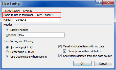
CUBERANKEDMEMBER (for Power Pivot slicers)
The CUBERANKEDMEMBER function returns an array of selected items and hence needs to be into as many (vertical) cells as you expect will be selected in the slicer. See the screenshot below.
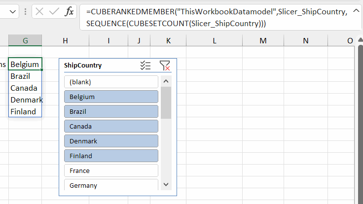
The formula is:
=CUBERANKEDMEMBER("ThisWorkbookDatamodel",Slicer_ShipCountry,SEQUENCE(CUBESETCOUNT(Slicer_ShipCountry)))
Note, that this is a dynamic array formula that only works in Excel 365. For older versions you should use a formula like the one below and copy that formula down far enough:
=IFERROR(CUBERANKEDMEMBER("PowerPivot Data",Slicer_Name,ROW()-ROW($G$2)),"")
The UDF
The code sample below must be placed in a normal module:
Dim oSc As SlicerCache
Dim oSi As SlicerItem
Dim lCt As Long
On Error Resume Next
Application.Volatile
Set oSc = ThisWorkbook.SlicerCaches(SlicerName)
If Not oSc Is Nothing Then
For Each oSi In oSc.SlicerItems
If oSi.Selected Then
GetSelectedSlicerItems = GetSelectedSlicerItems & oSi.Name & ", "
lCt = lCt + 1
End If
Next
If Len(GetSelectedSlicerItems) > 0 Then
If lCt = oSc.SlicerItems.Count Then
GetSelectedSlicerItems = "All Items"
Else
GetSelectedSlicerItems = Left(GetSelectedSlicerItems, Len(GetSelectedSlicerItems) - 2)
End If
Else
GetSelectedSlicerItems = "No items selected"
End If
Else
GetSelectedSlicerItems = "No slicer with name '" & SlicerName & "' was found"
End If
End Function
The function takes the slicer name as its argument and returns a text string (comma delimited) containing the selected items. In a worksheet cell the formula would look like this:
=GetSelectedSlicerItems("Slicer_TeamID2")
Conclusion
Well, I hope I got you started with getting your head around how slicers work and how to address them using VBA. I find Slicers a real gem in Excel. A great addition to the product!
Sample files
Download sample Excel workbooks 29 Aug 2019.
Other sources
Wall Street Oasis - Slicer in Excel: Tool Guide - Images and Video Instructions in Excel

Comments