Showing a picture from a list of pictures

Content

• Introduction
• Preparing the list
• Preparing the sheet that shows the dynamic picture
• Creating the picture
• Making the picture dynamic
• Download
• Other solutions

Introduction

Many people keep part lists in Excel. Sometimes even with embedded pictures next to the part data.

This article demonstrates a method to show a picture on a sheet that changes when a different part number is chosen from the list of available part numbers.

Preparing the list

The first thing to do is to position the pictures properly. Each picture should go in a cell on the same row as a unique description (part number) of the part it pertains to.

Format the cells, so the picture fits in a single cell (either adjust the size of the picture, or adjust row height and column width):

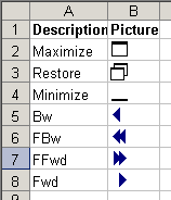
Figure 1, screenshot showing a list of icons next to their description

Preparing the sheet that shows the dynamic picture

We need some way of knowing which picture is to be shown. We start off by defining a dynamic range name that will expand automatically when we add new items to our list (assuming they are on Sheet1, starting on cell A1, with one row of headings) Choose Insert, name define (In Excel 2007 and up on the "Formulas" tab of the ribbon, in the "Defined Names" group, click the "Define Name" button) and define this name:

Let us say cell A2 on sheet2 will be used to enter the picture code we want to see the picture from. The formula in the next defined name will point to the cell to the right of the cell who's picture name matches the text entered in cell Sheet2!A2:

Creating the picture

Excel 2007

There are two methods to insert the proper picture in Excel 2007. One is by adding the camera tool to your QAT and using that, the other is shown below.

Select the cell where you want your dynamic picture to appear and click the Insert tab of the ribbon.  On the far right, find the "Object" button and click it (see screenshot below).

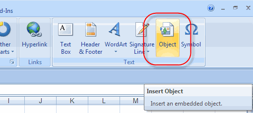
Figure 2, Insert Object button on the ribbon

The Insert object dialog appears:

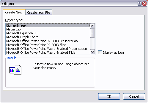
Figure 3, Object Dialog

Select the top option (Bitmap Image) and click OK.

Excel 2010

In Excel 2010, the Object button does not work, you have to either use the camera tool, or insert a picture from file (ane pciture file will do), after which you can change the formula.

After inserting the picture or object, hit escape to return to Excel. The newly inserted picture object should still be selected. The formula bar should show something like =EMBED("Paint.Picture";""). Click in the formula bar and replace the entire formula with this formula: =Picture

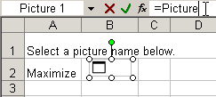
Figure 4, screenshot showing the picture's formula bar.

Hit enter or click the green checkmark to the left of the formula bar.

Excel 97 to 2003

Select the cell with the topmost picture. Hold down the shift key and click the Edit menu. It should show "Copy Picture...":

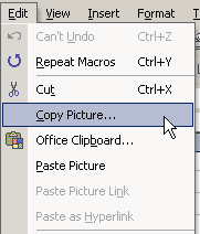
Figure 4, screenshot showing part of Excel's Edit menu when clicked whilst holding down the shift key.

Select "As shown on screen" from the next dialog and click OK.

Now navigate to the cell (on Sheet2 in this example) where you want to show the dynamic picture and hit the paste button (or control-v):

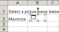
Figure 5, screenshot showing the pasted picture.

• This picture -of course- is static. To make it dynamic, we can use a formula as the source of the picture.
• Click on the picture so it is selected. Then click once in the formula bar:
  

Figure 6, screenshot showing the pasted picture's formula bar.

• Type the equal sign, followed by the name "Picture", as shown above and hit the enter key.
• Now select cell A2 and type one of the descriptions from the list into that cell. The picture belonging to that description should appear.

Making the picture dynamic

To simplify the selection of the picture description, we can use Data, validation:

• Select cell A2 and choose Data, Validation... from the menu.
• From the top dropdown, select the List option
• In the Source box enter this formula: =PictureList
• If needed, fill in the fields on the other tabs too ("Input message" and "Error Alert")
• Click OK:

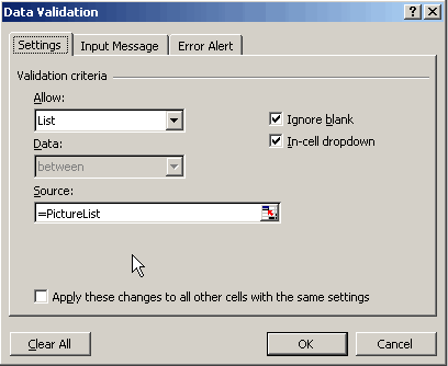
Now you can select from the available picture descriptions:

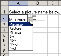
And we're done!

Download

Click here to download a sample file.

Other solutions

Bernie Deitrick came up with this nice sheet, which handles more pictures, but uses VBA