Creating A Simple Inventory System in Excel

Content

• Introduction
• Functionality
• Used techniques
• How its made
• The end result

Introduction

Answering questions on forums can be very rewarding. This post is the result of a forum question. The forum member needed a simple system to manage his shop inventory. He wanted to be able to log Purchases, Reservations and Sold items and immediately be kept informed when items are (almost) out of stock.

I built a very simple Excel file with just a handful of formulas, Validations and conditional formatting to do just that. Download the file from here: SimpleInventorySystem.zip

Functionality

The simple inventory system I built enables you to:

• Enter articles you sell
• Enter sold items
• Enter purchased items
• Enter reservations

It informs you of:

• Current stock for each item
• whether an article reaches a certain minimum stock level

Used techniques

I used these built-in functionalities of Excel:

• Tables
• Conditional formatting
• Formulas
• Data Validation

How its made

The tool has these worksheets:

Worksheet Articles

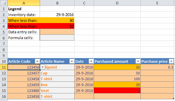
The Articles worksheet looks like this:

At the top B2 is an important cell because it holds the date which is used to calculate the stock levels. If you want stock levels to be up-to-date, make sure you have this formula in that cell: =TODAY()

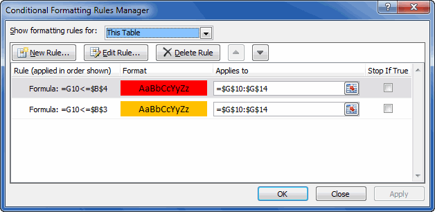
Cells B3 and B4 are used by conditional formatting formulas to visually indicate whether a product is close to going out of stock. If current stock is less than or equal to B3 the cell turns orange. If less than or equal to B4 it turns red.

Below the legend and settings cells the source table (named tblArticles) is located which contains all available products. In this table only the first three columns (the pale orange ones) are to be used for data entry.

Formulas

As you can derive from the formatting (the cells with white background and orange font color), columns D:G contain formulas. Lets study them.

Column D simply counts the number of items that have been purchased up to and including the date in cell B2:

=SUMIFS(tblPurchases[Purchased amount],tblPurchases[Article Code],[@Article Code],tblPurchases[Date],"<="&$B$2)

In Plain English: Sum the values of each row of column "Purchased amount" in table tblPurchase, provided that:

• The Article code in that table (tblPurchases[Article Code]) matches the article code in the current row ([@Article Code])
• The purchase date (tblPurchases[Date]) is less than or equal to the date in cell B2 ("<="&$B$2)

Columns E and F contain similar formulas to calculate how many items of this article have been reserved or sold respectively:

=SUMIFS(tblReservations[Reserved amount],tblReservations[Article Code],[@[Article Code]],tblReservations[Date],"<="&$B$2)

=SUMIFS(tblSales[Amount sold],tblSales[Article Code],[@[Article Code]],tblSales[Date],"<="&$B$2)

And finally column G calculates the current stock using some simple subtraction:

=[@Purchased]-[@Reserved]-[@Sold]

Validation rules

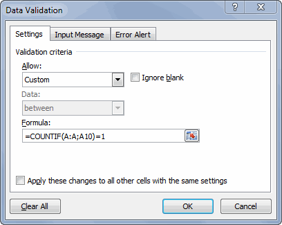
Column A of the table has Data, Validation setup to avoid duplicate article code entries. The screen-shot below shows the rule for cell A10:

Note: I have Dutch settings so the argument separator shown here is the ; instead of the ,

Conditional formatting

Column G has two conditional formatting rules applied to it, which ensure the cells change color if their inventory level reaches certain set values. The Conditional Formatting rules are:

Worksheet Reservations, Purchases and Sales

These three sheets have a very similar setup. This is a screenshot of worksheet Purchases:

Data Validation

Only column A contains a data validation rule:

It makes sure you can only enter (or select) article numbers from the ones on the Articles worksheet.

Conditional Formatting

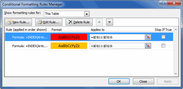
Similar to column G of the Articles sheet, column D contains Conditional Formatting rules:

The formula used is slightly more complex:

=INDEX(Articles!$G$10:$G$14,MATCH(A11,Articles!$A$10:$A$14,0))<=Articles!$B$4

So it looks at the table on the Articles sheet to find the current stock for the article in cell A11. If that amount is less than or equal to cell B4 on the articles sheet, the cell turns red.

This way, you'll be warned immediately whether the article you're adding to the Purchases, Sales or Reservations table is (almost) out of stock.

The end result

You can download the end result from here: SimpleInventorySystem.zip

That's all folks!