Fitting curves to your data using least squares

Content

• Introduction
• Fitting simple linear equations
• Fitting more complex functions
• Explanation of the Example file
• Conclusion

Introduction

If you're an engineer (like I used to be in a previous life), you have probably done your bit of experimenting. Usually, you then need a way to fit your measurement results with a curve. If you're a proper engineer, you also have some idea what type of equation should theoretically fit your data.

Perhaps you did some measurements with results like this:

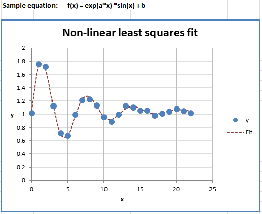
Fitting data with an equation.

A well known way to fit data to an equation is by using the least squares method (LS). I won't repeat the theory behind the method here, just read up on the matter by clicking that link to Wikipedia.

Fitting simple linear equations

Excel provides us with a couple of tools to perform Least Squares calculations, but they are all centered around the simpler functions: simple Linear functions of the shape
y=a.x+b, y-a.exp(b.x), y=a.x^b and etcetera. With some tricks you can also perform LS on polynomes using Excel.

Regression tools in the Analysis Toolpak Add-in

Activate the Analysis Toolpak in your list of Add-ins (File button or Office button, Excel Options, Add-ins tab, click Go):

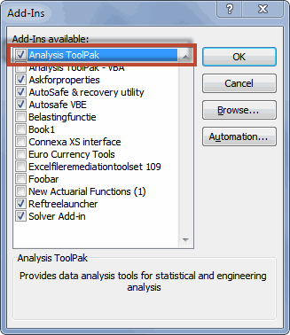
The add-ins list of Excel with the Analysis toolpak activated

This adds the "Data Analysis" button to your ribbon, on the Data tab, Analysis group (this is also the location where you can find the Solver button mentioned later on):

Ribbon with Data Analysis button

Click that button to explore which regression tools are available.

Worksheet functions

There is a number of worksheet functions which you can also use to do regression analysis. To quickly access them, select an empty cell and click shift+F3 to open the function wizard. In the search box, enter "Regression" (without the quotes of course). Excel will list the relevant functions:

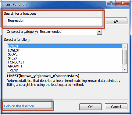
Function wizard showing Regression functions

Pick one and click on the "Help on this function" link at the bottom of the function wizard to find out more about its use.

Fitting more complex functions

What if you want to fit a more complex function, like y=exp(a.x).sin(x) + b ? How can that be done using Excel?

I devised a way to do this which involves the following steps:

• Create a table with x and y values
• Add a column with the model function formula, which points to your x-es and to some cells for the constant(s)
• Have a column that calculates the Sum of Squares
• Use Solver to find the constants which yield the lowest Sum of Squares.

Explanation of the Example file

I created an example file you can put to use directly. Below you will find a link to the file and an explanation on how the file is put together.

Download

Download this file:

Non linear least squares example

How the file works

Data

The calculations and the data are concentrated on Sheet1 of the file. The most important area is the table starting in cell A1:

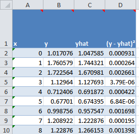
Data table in LS file

Column A holds your x-values and column B holds the y-values. The third column holds the formula that calculates the result of the fitted equation using the constants and the x-values. The sample file has this formula in column C:

=EXP(Const_a*xValues)*SIN(xValues)+Const_b

The fourth column of the table is used to calculate the sum of squares. Formula:

=(B2-C2)^2

As you probably noted already, I used a couple of range names. I explain those below.

Range names

To ease working with the file I created some range names. Instead of using the table references that current Excel offers, I included some dynamic range names that point to the data.

Constants of the equation

The const range names point to a second table in the file:

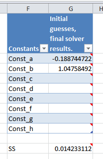
Constants table

This table is where you enter your first initial guesses for the resulting constants and where the Solver add-in also returns the results. As you can see, below that table the residual Sum of Squares is shown. Formula:

=SUM(yDelta)

It is this cell G11 that we try to minimize using the Solver add-in.

Using Solver

First of all, you need to install the Solver add-in. Use the Add-ins dialog I showed at the top of this article and check the box next to "Solver Add-in". This adds the Solver button in the same location on the ribbon as the "Data Analysis" button I showed before.

After you have ensured the model formula is correctly entered in column C and the calculations work, click the Solver button. The dialog below is shown:

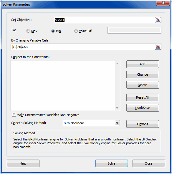
The Solver dialog

Make sure the "Set Objective" box points to the cell that contains the sum of squares. Select "Min" next to "To".

The "By Changing Variable cells" box must ONLY point to the cells that are used by your model, otherwise the degrees of freedom calculation (on the ANOVA sheet) will be wrong. Also ensure that any unused constant cells are empty by selecting them and hitting the del key.

Note that depending on your model type you may have to change the solver settings. A bit of experimenting may be needed for best results. You can save and load Solver settings using the appropriate button.

So be prudent and critical on whether or not you have actually reached a best fit, the Solver may come up with non-optimal results, depending on your model equation and solver settings.

If you're happy with the current Solver settings, click Solve. After some time the "Solver Results" dialog opens, giving you some options on how to continue. Note that it also enables you to ask for a couple of reports.

The example file shows the end result:

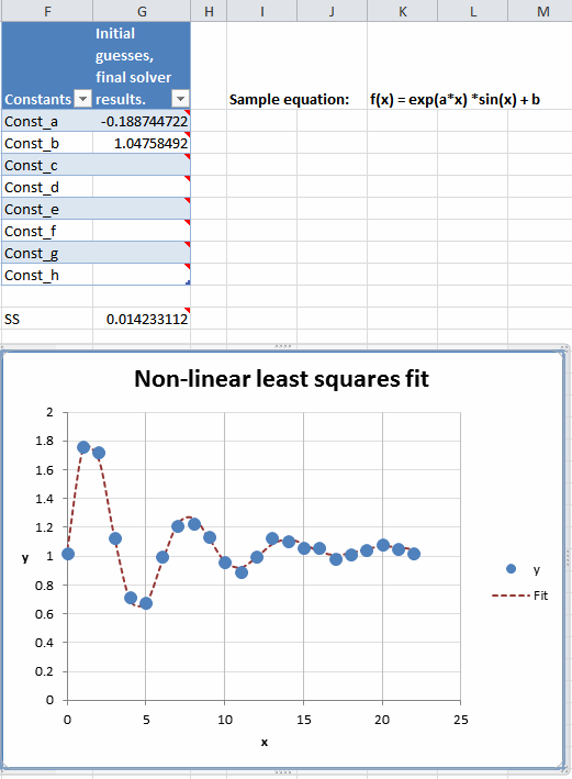
The end result

Analysis of Variance

Below the chart, you can find the ANalysis Of VAriance table, which looks like this:

The ANOVA table

The most important cell here is cell K34. If the value in that cell is less than 0.05, there is a 95% probability your model is correctly fitting the data. So less is more for this cell, you want it to stay below 0.05. The cell will turn red for values over 0.05.

Please check whether the value in cell G34 is exactly one less than the number of constants you used for the model. If not, go back to Sheet1 and empty the cells not used by your model. So if you used const_a and const_b, then the value of G34 (model degrees of freedom) should be 1.

Conclusion

As you've seen fitting complex functions to your data isn't very hard to do. A combination of some relatively simple formulas and the Solver Add-in comes to the rescue here.

Some advice as one engineer to another; Be critical please. Don't believe everything Excel tells you! Carefully analyse the results it returns, as Solver may get things wrong and not give you the best possible result!