
Excel Office Script Examples
Content
- Introduction
- Video
- Entering zeroes in empty cells
- Last Used Row
- Adding a table of Contents to your workbook
- Adding a list of Range names
- Prompting for user input
- Filter a table by date
- Sending email using Office Script
- Download
Introduction
Since July 2020, Microsoft 365 users can record their actions in Excel on-line into Office Script macros. Earlier, I've posted an article that shows you how to get started. On this page, I will list some example scripts which you cannot record but might come in handy.
Some of these scripts contain literal values, (the values between quotes). This means things like worksheet names are hard-coded into the example scripts: "ToC". So if you need a different worksheet name, edit the script accordingly. Because Microsoft has not yet given us a way to prompt the user for a value, we must edit the script to change what sheet it affects.
Download the full code (zip file with all scripts) here.
Video
I've presented parts of this page during Excel Virtually Global 2022. Here's the Youtube recording:

Entering zeroes in empty cells
Suppose you want to enter a zero in each empty cell in the selection:
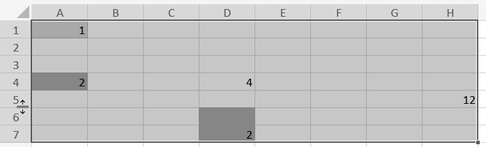
This code does exactly that.
Last Used Row
The function getLastRow shown below, returns the last used row of any range (assuming the cell on row 1048576 is empty!)
Notice that the script will return a string instead of a number if the last cell of the sheet contains something. This will cause an error in the calling routine which you must handle.
Adding a table of Contents to your workbook
Working in Excel Online and need a table of Contents for your workbook quickly? Here's an Office Script that produces one. It generates a list for all worksheets and all charts, with hyperlinks pointing to their locations.
First let me show the main function and explain it step by step.
These are the important steps in this code:
- check whether a worksheet called ToC exists and if it does, delete it.
- Fetch a list of all worksheets and store that in a variable called allSheets
- Add a worksheet called "ToC" and assign it to a variable called tocSheet
- Assign cell B2 to the variable reportCell
- Add a table to the table of contents using the function addTocTable (see below)
- To ensure we start adding the sheet names on the first empty row of the table, we offset the reportCell with two so it now points to cell B4
- We add the headings (Worksheet and Link) to the newly inserted table
- Now it is time to loop through the allSheets collection and list the name of each sheet in the first column of the table
- After looping through the sheets, we add the HYPERLINK formula to the second column, using the name of the worksheet in the first column to create a link to each worksheet
- We offset the reportCell position by adding the number of rows in the worksheet table (plus two rows extra for spacing)
- Now we add the heading for the charts table and an empty table to hold them, using that addTocTable function again
- The Charts table has four columns: Worksheet, Name, Location and Link
- We run through all worksheets and for every worksheet we
- run through all charts
- fill the chart table with the appropriate information: Worksheet, Name and Location (location required me to design a function called getCellUnderChart because Office Script does not have a TopLeftCell property of a chart like VBA has)
- There's a snag for charts on sheets which contain a space in their name; the correct address of the topleftCell in sheets like that have apostrophes around the name: 'Blad 2'!F1. However, if you write 'Blad 2'!F1 to a cell, Excel strips that first apostrophe. Hence the if statement that adds an additional apostrophe in such cases.
- Once we've done all charts on all worksheets, we place the HYPERLINK formula in the last column again using the address information in the third column
The main function uses two helper functions, here's the addTocTable one:
All it does is add the caption in the location cell, style it as "Heading 1" and add a new one-column table. The function returns the table as an object so we can use that object in our calling routine.
Note that you can also address a style by its name. But be aware that built-in style names are language-dependent. So only assign a style by its name if it is a custom style.
And here is the getCellUnderChart function:
The basic principle is simple: the function first loops through the cells of the worksheet horizontally, starting from cell A1, until it has found a cell with a Left value that is greater than or equal to the chart's Left position. After that it does the same vertically to find the Top position. Because the two loops take us one column too far to the right and one row too far down, we offset the found cell by (-1, -1) so we return the correct cell which denotes where the top-left corner of the chart is located.
Adding a list of Range names
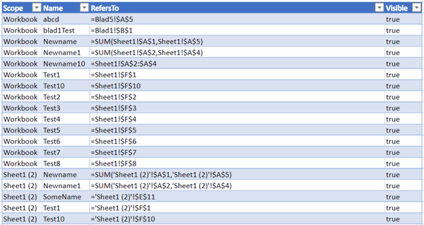
Desktop Excel has a simple feature to add a list of range names to your workbook (Formulas tab, Use in Formula drop-down, Paste List). But Excel on-line does not (yet) have that feature. Here is an Office script which adds a worksheet called "Names List" to your workbook, listing all range names and some of their properties.
The resulting table looks like this:
Prompting for user input
OfficeScript does not have a feature like the VBA InputBox, nor can you design input screens.
Recently, Microsoft has provided a way to solve that issue. If you add input parameters to your function definition, Excel will show a little prompt window asking for their values. It will even add space characters before each capitalized letter of your variable name. Take this script for example:
If you execute this script, this is what is shown:
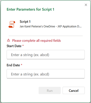
There is some intelligence to this. If a parameter is a boolean, it will present a drop-down with true/false. And you can set default values too. In addition, I wanted to define the StartDate and EndDate parameters as "Date", but apparently that isn't a valid data type for TypeScript. I was hoping it'd recognize this and offer me a date picker. O well, at least we can prompt the user for input values.
Alternative to using arguments
If you need more elaborate input, perhaps this offers some help.
The script below checks for presence of a worksheet called "Script_Input". If that sheet is not in the workbook, it gets added. Next a function is called which allows you to pass it a prompt and an array of inputs, which will be added to the Script_Input sheet. The resulting input sheet looks like this:
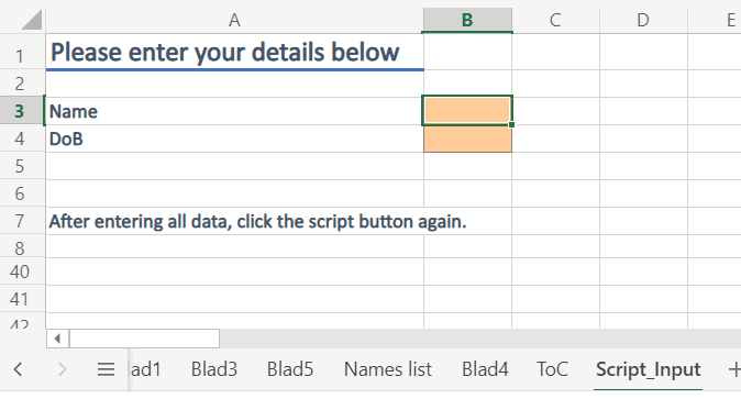
If the script detects that the "Script_Input" sheet is available, it assumes all input has been completed and runs an action with that input (writes to the console).
This is the entire script:
Filter a table by date
Suppose you have a table with a date column and you want to filter that table by dates prior to today.
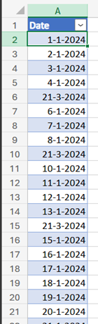
To make this happen, you need the proper date format which applies to your Excel settings; is it mm/dd/yyyy or dd-mm-jjjj? For this you use the so-called cultureInfo of the Excel application:
workbook.getApplication().getCultureInfo().getName()
This returns a string in the shape en-US or (in my case) nl-NL. This string can then be used to convert the current system date to the proper locale string.
To filter this table for dates prior to today, you use code like this:
You can also use the ISO date format, which should work too:
Sending Personalised PDF Reports with Office Scripts
In this example, we'll build an Excel workbook that automatically generates and emails a personalised PDF report to every recipient listed in a table. The solution uses the new Office Scripts PDF and email capabilities, allowing Excel to create PDF attachments and send emails without relying on Outlook VBA automation.
The workbook is driven by a table named tblAddresses. Each row represents a recipient. The table contains at least two columns:
| Column | Purpose |
|---|---|
| ID | Unique identifier used to personalise the report. |
| Recipient's email address. |
For each row in the table, the script writes the value from the ID column into a workbook-level named range called Email_id. This named range acts as the driver for the report and can be used in formulas, or any other workbook logic needed to generate recipient-specific content.
The workbook also contains a worksheet named Email_attachment. This worksheet serves as the report template. Its contents can reference Email_id directly or indirectly through formulas, allowing the worksheet to automatically display the information relevant to the current recipient.
Two additional workbook-level named ranges control the email content:
| Named Range | Purpose |
|---|---|
| Email_subject | Contains the email subject line. |
| Email_body | Contains the email body text. |
| Email_id | Contains the current recipient ID. |
Because the script recalculates the workbook after updating Email_id, both Email_subject and Email_body may contain formulas that dynamically generate personalised text for each recipient.
The overall process works as follows:
- Read all records from tblAddresses.
- For each recipient:
- Write the recipient's ID to Email_id.
- Recalculate the workbook.
- Read the contents of Email_subject and Email_body.
- Convert the worksheet Email_attachment to PDF.
- Send an email to the address stored in the email column using Email_subject as the subject line and Email_body for the body.
- Attach the generated PDF report to the email message.
- Repeat until all recipients have received their personalised report.
This design keeps all business logic inside the workbook. Email recipients are controlled from tblAddresses, report generation is controlled by Email_attachment, and the email text is maintained through the named ranges Email_subject and Email_body. No hard-coded recipient lists, subject lines, or message text are required in the script itself, making the solution easy to maintain and update by workbook authors rather than developers.
Here is the entire script for your reference (also included in the download of course):
Download
Download the full code (zip file with all scripts) here.
Next article: Call a script from a Power Automate Flow
In my next article I describe how to apply the Table Of Content script to all Excel files in a Sharepoint folder using Power Automate
Frequently asked Questions
What is Office Script in Excel and since when has it been available?
How can I enter zeroes in empty cells using an Office Script?
How do I find the last used row in a column with Office Script?
How can I add a table of contents to my Excel workbook using Office Script?
Is there a way to list all range names in Excel Online using Office Script?
Where can I find a video presentation about these Office Script examples?
How does the addTocTable function work in creating a table of contents?
What is the purpose of the getCellUnderChart function in the table of contents script?
What happens if the last cell in the column is filled when using the getLastRow function?
Why do some scripts require editing hard-coded worksheet names?
Comments