 Back to jkp-ads.com |
Ron de Bruin
|
|
|
Back to jkp-ads.com |
Ron de Bruin
|
|
Ron de Bruin decided to remove all Windows Excel content from his website for personal reasons. If you want to know why, head over to rondebruin.nl.
Luckily, Ron was kind enough to allow me to publish all of his Excel content here.
Most of these pages are slightly outdated and may contain links that don 't work. Please inform me if you find such an error and I'll try to fix it.
Kind regards
Jan Karel Pieterse
You can find the information from this page also in my MSDN article:
http://msdn.microsoft.com/en-us/library/cc952296.aspx
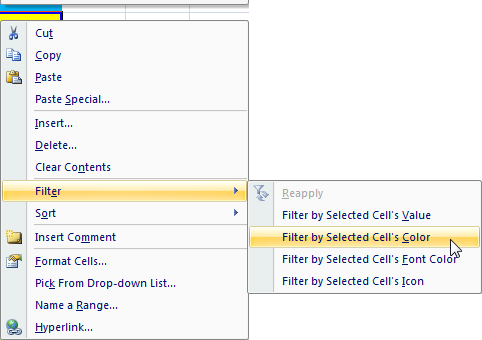
In Excel 2007-2016 there are new commands on the
Cell menu that make it easy to filter a table based on the active
cell's value, font color or fill color.This article discusses how you can
access these features with a macro.
The Cell menu is
the menu that pops up when you right click a cell:
Note: There are two ways that a cell's font or fill
color can be set. One is by the Fill and Font controls in the Font group on
the Home tab. The other is by Conditional Formatting in the Styles group on
the Home tab. The great thing about the new color filtering features is that
it works with colors set either way.
When you select one of the
filter options on the Cell menu Excel will guess what your filter range is
if you've selected only a single cell. If you have any empty rows in your
table Excel may not select the range you intend.
In the basic example below I show how to use one of the built-in options
in your VBA code using the Commandbars Execute method. Why not use the Range
AutoFilter method instead?
The problem with the AutoFilter method is that
it requires you to specify the font or fill color of the active cell. That's
easy to do when the colors are set by the Font group controls, but when the
colors are set because of Conditional Formatting it is impractical, if not
near impossible, to do.
Why? Because Excel does not
give us a direct way to tell in code what font or fill colors a cell is
displaying as a result of conditional formatting. Our code would have to
work through the conditional formatting rules and figure out the one in
effect, if any, and then figure out the formatting applied, if any. It is
much easy to use the Execute method and have Excel do all this work.
The code example will create a new worksheet or workbook with every record
with the same Fill interior Color/Pattern or Shading style of the active
cell.
You can change the number in this part of the macro if you want
to filter on the font color or value.
'Call the built-in filter option to filter on ACell
Application.CommandBars("Cell").FindControl _
(ID:=12233, Recursive:=True).ExecuteControl
12232 = Filter by Selected Cell's Value
12233 = Filter by Selected Cell's
Color
12234 = Filter by Selected Cell's Font Color
12235 = Filter by
Selected Cell's Icon
Why do I use the Control Id instead of the control caption ?
If you
use the ID the code will work in every language version of Excel
Tip: See also the tips part below the macro on this page.
Maybe there is something useful there for you if you want to change the
code.
In my example code I filter on the Fill interior color/Pattern or Shading
style.
Select a cell with a Fill interior color/Pattern or Shading
style and Run the macro. The macro will create a new worksheet for you with
the filter results. Every time you run the code it will delete the worksheet
first so you are sure that the worksheet have the latest filter results.
Read this part in the macro good "Optional set the Filter range".
If there are empty rows or columns in your data in a normal range you can
make sure that Excel uses the correct data range in this code part.
Sub Filter_Example_Excel_2007_2016()
    Dim ACell As Range
    Dim WSNew As Worksheet
    Dim Rng As Range
    Dim ActiveCellInTable As Boolean

    With Application
        .ScreenUpdating = False
        .EnableEvents = False
    End With

    'Delete the sheet MyFilterResult if it exists
    On Error Resume Next
    Application.DisplayAlerts = False
    Sheets("MyFilterResult").Delete
    Application.DisplayAlerts = True
    On Error GoTo 0

    'Remember the activecell
    Set ACell = ActiveCell

    'Test if ACell is in a Table or in a Normal range
    On Error Resume Next
    ActiveCellInTable = (ACell.ListObject.Name <> "")
    On Error GoTo 0

    'Optional set the Filter range
    If ActiveCellInTable = False Then
        'Your data is in a Normal range.

        'If there are empty rows or columns in your data range you
        'can make sure that Excel uses the correct data range here.
        'If you do not use these three lines Excel will guess what
        'your range is. Here we assume that A1 is the top left cell
        'of your filter range and the header of the first column and
        'that C is the last column in the filter range

        '        Set Rng = Range("A1:C" & ActiveSheet.Rows.Count)
        '        Rng.Select
        '        ACell.Activate
    Else
        'Your data is in a Table

        'No problem if there are empty rows or columns if your data.
        'is in a Table so there is no need to set a range because
        'it automatically uses the whole table.
    End If


    'Call the built-in filter option to filter on ACell
    Application.CommandBars("Cell").FindControl _
            (ID:=12233, Recursive:=True).Execute

    'Control Id     Description
    '12232          Filter by Selected Cell's Value
    '12233          Filter by Selected Cell's Color
    '12234          Filter by Selected Cell's Font Color
    '12235          Filter by Selected Cell's Icon

    ACell.Select

    'Copy the Visible data into a new worksheet
    If ActiveCellInTable = False Then
        On Error Resume Next
        ACell.Parent.AutoFilter.Range.Copy
        If Err.Number > 0 Then
            MsgBox "Select a cell in your data range"
            With Application
                .ScreenUpdating = True
                .EnableEvents = True
            End With
            Exit Sub
        End If
    Else
        ACell.ListObject.Range.SpecialCells(xlCellTypeVisible).Copy
    End If

    'Add a new worksheet to copy the filter results in
    Set WSNew = Worksheets.Add
    WSNew.Name = "MyFilterResult"

    With WSNew.Range("A1")
        .PasteSpecial xlPasteColumnWidths
        .PasteSpecial xlPasteValues
        .PasteSpecial xlPasteFormats
        Application.CutCopyMode = False
        .Select
    End With

    'Close AutoFilter
    ACell.AutoFilter

    With Application
        .ScreenUpdating = True
        .EnableEvents = True
    End With

End Sub
Tip : Create a new workbook instead of a worksheet
If you want to create a new Workbook with the filter results instead of a
Worksheet then :.
Delete this part
        'Delete the sheet MyFilterResult if it exists
        On Error Resume Next
        Application.DisplayAlerts = False
        Sheets("MyFilterResult").Delete
        Application.DisplayAlerts = True
        On Error GoTo 0
And replace this line
Set WSNew = Worksheets.Add
With
Set WSNew = Workbooks.Add.Worksheets(1)